TopoPoint — Enhance Topology Reasoning via Endpoint Detection in Autonomous Driving
Paper review · endpoint를 명시적으로 detection하자.
각 figure의 출처는 하이퍼링크로 달아두었습니다 :)
+++ Lane Topology Reasoning 섹션의 다섯 번째 글이다. TopoLogic은 “lane–lane이 안 풀리는 진짜 이유는 endpoint shift”라고 진단하고, 해당 shift를 distance function을 정의하여 SGNN(message passing)에 반영하는 방식으로 해결하려 했다. TopoPoint는 같은 진단에서 정반대로 간다. “어긋나는 걸 message passing에 반영하는 식의 간접적인 방식말고, endpoint 자체를 따로 검출해서 supervision을 줘버리자.” TopoLogic과 같은 저자(ICT, CAS)의 직속 후속작이고, 코드도 TopoLogic의 그 sgnn_decoder.py를 그대로 물려받는다.
TopoPoint: Enhance Topology Reasoning via Endpoint Detection in Autonomous Driving
Authors : Yanping Fu, Xinyuan Liu, Tianyu Li, Yike Ma, Yucheng Zhang, Feng Dai (ICT, Chinese Academy of Sciences · Shanghai AI Lab)
Venue : NeurIPS 2025
Paper Link : https://arxiv.org/abs/2505.17771
Code : https://github.com/Franpin/TopoPoint (공식)
Introduction & Motivation
endpoint deviation — TopoLogic이 implicit하게 해결한 문제
TopoLogic 글에서 봤듯, lane–lane topology가 바닥을 기는 핵심 원인은 endpoint shift였다. 두 lane이 이어진다는 건 한 lane의 끝점과 다음 lane의 시작점이 같은 자리에 있다는 뜻인데, lane들은 서로 다른 query에서 독립적으로 regression되니 그 두 점이 정확히 겹친다는 보장이 없다. GT에선 맞닿아 있던 끝점이 예측에선 미묘하게 어긋나고, 그 어긋남이 topology를 망친다.
TopoPoint의 진단은 한 줄 더 들어간다. endpoint가 lane query에 딸려 나오는 auxiliary라는 게 문제의 뿌리다. lane query 하나가 centerline 전체를 regression하고, 그 양 끝이 곧 endpoint가 된다. 그러니 endpoint는 lane 전체를 맞추려는 supervision에 휩쓸려 정확도가 떨어지고, 여러 lane의 endpoint들이 한 점에 모여야 할 때 제각각 흩어진다.
TopoLogic은 이 endpoint shift 문제를 거리가 충분히 가까우면 연결로 판단하는 geometry kernel 함수를 정의하여, SGNN에 반영해 topology에 geometry(특히 endpoint) 정보를 주입했다. TopoPoint는 어떻게 보면 정반대다. endpoint를 lane에 딸린 auxiliary가 아니라, lane과 나란히 검출되는 하나의 객체로 끌어올린다.
endpoint를 따로 검출하면 무엇이 좋은가
endpoint를 독립 query로 두면 두 가지가 생긴다.
- endpoint가 lane 전체 supervision과 분리되어 자기 위치만 집중해서 맞춘다 — endpoint 정확도 자체가 올라간다.
- 검출된 point와 lane을 서로 맞춰, lane의 끝점을 point 쪽으로 끌어당겨 deviation을 줄일 수 있다.
이를 위해 TopoPoint는 세 가지를 얹는다.
- Point-Lane Merge Self-Attention (PLMSA) — point query와 lane query를 합쳐, 둘 사이 geometric distance를 attention bias로 넣어 정보를 섞는다.
- Point-Lane Graph Convolutional Network (PLGCN) — point와 lane feature를 GCN으로 양방향 aggregation한다.
- Point-Lane Geometry Matching (PLGM) — inference 때 검출된 point로 lane endpoint를 보정하는 후처리.
그리고 endpoint 검출 품질을 재기 위해 $\text{DET}_p$라는 metric을 새로 제안한다. 아래에서 PLMSA·PLGCN·PLGM을 코드와 수식으로 본다.
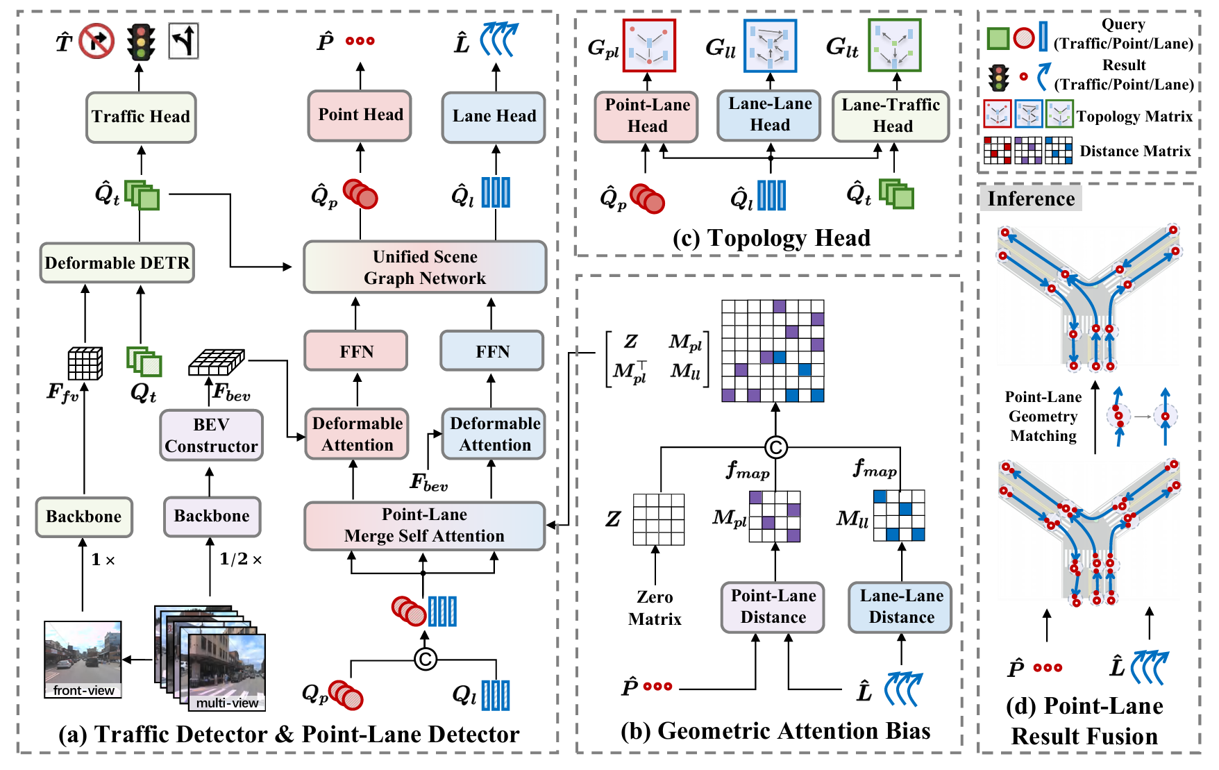
Method
전체 파이프라인 개요
골격은 시리즈의 다른 글들과 같은 BEV→DETR이되, query가 둘로 갈라진다.
- 멀티뷰 이미지를 BEVFormer로 BEV feature로 만든다.
- point query $Q_p$와 lane query $Q_l$를 독립적으로 초기화해, 각자 reference point로 deformable cross-attention을 태운다($N_p=200, N_l=300$).
- decoder layer 안에서 PLMSA → PLGCN으로 point·lane feature를 섞고, point head·lane head로 endpoint와 centerline을 regression한다.
- inference에서 PLGM으로 lane endpoint를 검출된 point에 맞춰 보정한다.
baseline은 TopoLogic이다 — 논문도 코드도 TopoLogic 위에 point 갈래를 얹은 형태다. 아래 ①②③을 보자.
① Point-Lane Merge Self-Attention — 거리를 attention bias로, point까지
point와 lane이 따로 검출되니, 둘이 서로를 봐야 한다. PLMSA는 두 query를 concat한 뒤 self-attention을 돌리는데, 그냥 돌리지 않고 point–lane, lane–lane 사이 거리를 attention bias로 더한다.
거리 행렬부터. lane–lane은 lane $i$의 끝점과 lane $j$의 시작점 거리($D_{ll}$), point–lane은 point $i$와 lane $j$의 시작/끝점 중 더 가까운 쪽 거리($D_{pl}$)다.
그리고 이 거리를 bias로 바꾸는 커널 함수 $f_\text{map}$가 TopoLogic의 그 함수 그대로다.
TopoLogic 글에서 “이게 정말 learnable이라 부를 만한가”를 길게 의심했던 그 $e^{-x^\alpha/(\lambda\sigma)}$다. 같은 저자가 같은 함수를 이번엔 topology score가 아니라 attention bias로 쓴다. 코드도 TopoLogic의 그 한 줄을 그대로 옮겼다 — 다만 lane용 $P, w$ 옆에 point용 $pt\_P, pt\_w$를 추가했을 뿐이다.
# projects/topopoint/models/modules/sgnn_decoder.py — forward()
# point–lane 거리: start/end 중 가까운 쪽 (= D_pl)
distance_1 = torch.sum(torch.abs(pt_tensor[:,:,:,0,:] - lc_tensor[:,:,:,0,:]), dim=3)
distance_2 = torch.sum(torch.abs(pt_tensor[:,:,:,0,:] - lc_tensor[:,:,:,-1,:]), dim=3)
ptlc_distance = torch.min(distance_1, distance_2)
ptlc_topo = torch.exp(-torch.pow(ptlc_distance, self.pt_P) / (self.pt_w))   # f_map, point용

# lane–lane 거리: 끝점↔시작점 (= D_ll), TopoLogic과 동일
topo = torch.sum(torch.abs(o1_tensor[:,:,:,-1,:] - o2_tensor[:,:,:,0,:]), dim=3)
topo = torch.exp(-torch.pow(topo, self.P) / (self.w)) * topo_mask           # f_map, lane용
이 bias들을 self-attention score에 더한다. concat한 query $Q_{pl}=[Q_p; Q_l]$에 대해, attention mask는 블록 행렬이다 — point–point 블록은 zero(거리 prior 없음), 나머지는 $M_{pl}, M_{ll}$다 (paper Eq. 기준).
🤔 (사견) T2SG와 거의 같은 그림인데, 분리한 게 차이다. 거리를 attention bias로 더한다는 골격은 바로 앞 글 T2SG의 $A_\text{SPM}$과 사실상 같다. (음… T2SG가 arXiv에 최초 공개된게 2024년 11월인걸 생각해보면, 인용은 안 했지만 뭔가 본게 아닐까?) 차이는 TopoPoint가 point–point/point–lane/lane–lane을 블록으로 쪼개고, point–point는 아예 bias를 안 준다(zero)는 점이다. point끼리는 기하적으로 가깝다는 게 별 의미가 없으니(같은 교차로의 두 endpoint가 가까운 건 당연하다) 거리 prior를 빼버린 것으로 읽힌다. T2SG가 lane만 있는 한 종류의 거리였다면, TopoPoint는 point를 끌어들이면서 “어떤 거리는 의미 있고 어떤 거리는 아니다”를 블록으로 구분한 셈이다.
② Point-Lane Graph Convolutional Network — point와 lane을 양방향으로
PLMSA가 attention으로 섞었다면, PLGCN은 GCN으로 한 번 더 섞는다. point–lane 인접 행렬을 만들어, point feature를 lane으로, lane feature를 point로 양방향 전파한다.
Adjacency matrix는 semantic topology와 geometric bias의 가중합이다 — TopoLogic의 “similarity + distance fusion”이 여기선 point–lane 버전으로 반복된다.
$G_{pl}$은 topology head가 낸 point–lane 의미 연결, $M_{pl}$은 ①의 geometric bias다($\lambda_1, \lambda_2$는 learnable, 둘 다 1.0 초기화). 이 인접 행렬로 GCN을 돌려 feature를 갱신한다.
코드에서도 이 fusion이 TopoLogic 구조 그대로다 — point–lane adjacency를 pt_lamda_1 * (sim adjacency).detach() + pt_lamda_2 * (geometric topo)로 만든다. similarity 쪽 gradient를 떼는 것까지 TopoLogic과 같다.
# projects/topopoint/models/modules/sgnn_decoder.py — forward()
ptlc_rel_adj = ptlc_rel_out.squeeze(-1).sigmoid()                        # G_pl (semantic)
prev_ptlc_adj = self.pt_lamda_1 * ptlc_rel_adj.detach() + self.pt_lamda_2 * ptlc_topo   # A_pl
③ Point-Lane Geometry Matching — inference 후처리로 endpoint 보정
마지막은 학습이 아니라 inference 단계의 후처리다. 검출된 point로 lane의 끝점을 끌어당겨 deviation을 직접 메운다.
알고리즘은 단순하다. confidence가 높은 point·lane만 남기고, 한 point 근처(거리 임계 $\delta=1.5$m 안)에 있는 lane endpoint들을 모은다. 그리고 그 point와 모인 endpoint들의 평균을 새 endpoint로 삼아, 관련 lane들의 끝점을 전부 그 한 점으로 덮어쓴다.
코드도 정확히 평균이다 — 한 lane의 끝점과, topology score가 임계를 넘는 이웃 lane들의 끝점을 모아 torch.mean으로 합친 뒤 덮어쓴다.
# projects/topopoint/models/dense_heads/topopoint_head.py — get_lanes()
mean_pts = torch.mean(torch.cat(pts, dim=0), dim=0)   # point + 이웃 endpoint들의 평균
select_lanes_preds_new[0, i, 0, :]  = mean_pts        # 시작점 덮어쓰기
select_lanes_preds_new[0, i, -1, :] = mean_pts        # 끝점 덮어쓰기
⚠️ 여기도 TopoLogic의 하드코딩이 그대로 따라왔다. 이 후처리 코드에
w = 11.5275가 상수로 박혀 있다 — TopoLogic 글에서 짚었던, 학습된 $w$를 inference에 하드코딩한 바로 그 값이다(초기값 10에서 수렴한 값). 같은 코드베이스를 물려받았으니 같은 상수가 그대로 넘어온 셈인데, point 갈래를 새로 붙이면서 이 값이 여전히 적절한지는 따로 확인된 바 없어 보인다.
🤔 (사견) PLGM은 TopoLogic의 plug-in 후처리와 같은 결이다. TopoLogic도 “학습 없이 거리로 topology를 보정하는 후처리”를 plug-in으로 내세웠다. PLGM은 그 후처리를 endpoint 좌표 자체로 옮긴 버전이다 — gradient 없이, inference에서 point로 lane 끝점을 평균내 덮어쓴다. ablation에서 PLGM의 기여는 $\text{DET}_p$ +0.8로 셋 중 가장 작은데(PLMSA +5.0, PLGCN +2.0), 무거운 일은 PLMSA·PLGCN이 학습으로 다 해놓고 PLGM은 마지막 마무리만 하는 구조다. 후처리가 작은 건 오히려 “학습 단계에서 이미 endpoint가 잘 모였다”는 것 아닐까.
④ Loss
loss는 traffic·point·lane 검출과 세 topology의 합이다 (paper Eq. 21).
point는 $\mathcal{L}_p$(focal + L1)로 lane과 똑같이 검출 supervision을 받는다. 별도의 endpoint 거리 loss는 없다 — endpoint는 그냥 GT point 위치로 regression될 뿐이고, “끝점을 모으는” 일은 PLMSA·PLGCN의 거리 bias와 PLGM 후처리가 맡는다. topology 항들($\lambda_{pl}=\lambda_{ll}=\lambda_{lt}=5.0$)이 검출 항(1.0)보다 무겁게 걸린다.
OpenLane-V2 Benchmark & Results
평가는 시리즈 그대로 OpenLane-V2, OLS에 endpoint 검출용 $\text{DET}_p$가 추가된다. subset_A 기준 paper Table 1.
| Method | $\text{DET}_l$ | $\text{DET}_t$ | $\text{TOP}_{ll}$ | $\text{TOP}_{lt}$ | OLS | $\text{DET}_p$ |
|---|---|---|---|---|---|---|
| TopoNet | 28.6 | 48.6 | 10.9 | 23.8 | 39.8 | 43.8 |
| TopoMLP | 28.3 | 49.5 | 21.6 | 26.9 | 44.1 | 43.4 |
| TopoLogic | 29.9 | 47.2 | 23.9 | 25.4 | 44.1 | 45.2 |
| TopoPoint | 31.4 | 55.3 | 28.7 | 30.0 | 48.8 | 52.6 |
- $\text{DET}_p$가 크게 오른다. 45.2 → 52.6으로 TopoLogic 대비 +7.4. endpoint를 일급 객체로 검출한 효과가 가장 직접적으로 드러나는 숫자다(애초에 이 논문이 새로 만든 metric이라 자기 강점이 부각되는 면도 있다).
- $\text{TOP}_{ll}$도 따라 오른다. 23.9 → 28.7로 +4.8. endpoint가 잘 모이니 lane–lane도 같이 올라간다 — TopoLogic의 진단(“endpoint가 topology의 병목”)이 맞다면 endpoint를 고치면 topology가 오르는 게 당연하고, 실제로 그렇게 나왔다.
- OLS는 44.1 → 48.8로 시리즈 최고다. 다만 이 숫자를 그대로 믿기 전에 $\text{DET}_t$(47.2 → 55.3)를 따로 떼어 봐야 한다. 아래 박스에서 다룬다.
⚠️ $\text{DET}_t$ +8은 모델이 아니라 입력 해상도 트릭이다. TopoPoint는 surround 6장(BEV용)은 0.5배로 줄이면서 traffic 검출에 쓰는 front-view 한 장만 full resolution으로 들고 간다. 논문도 명시한다 — “keeping the front-view at its original resolution.” 코드도 그대로다.
# projects/topopoint/datasets/pipelines/transform_3d.py — RandomScaleImageMultiViewImage
results['front_img'] = [results['img'][0].copy()]   # front-view는 원본(full-res) 그대로
results['img'] = [mmcv.imresize(img, (x_size[idx], y_size[idx]), ...) for ...]  # surround만 0.5배
ablation의 “FVScale” 한 줄이 정확히 이거고, front-view만 0.5 → 1.0으로 올리는 것만으로 $\text{DET}_t$가 46.8 → 53.8로 +7.0 튄다. OLS가 $\text{DET}_t$를 1/4 가중으로 직접 포함하니, 이 입력 해상도 하나가 OLS를 ~+1.75 밀어올린다. endpoint 검출이라는 본 줄기와는 아무 상관이 없는, 순수하게 “traffic 쪽 입력을 더 크게 넣은” 이득이다.
더 걸리는 건 비교 방식이다. Table 1의 TopoNet·TopoMLP·TopoLogic 수치는 원 논문에서 그대로 가져온 것이지(DET$_p$만 official code로 따로 계산), 이 full-res front-view 세팅으로 다시 돌린 게 아니다. 즉 TopoPoint만 traffic 입력을 풀 해상도로 키운 채, 그 이점이 없을 수도 있는 다른 모델들과 $\text{DET}_t$를 나란히 세워 놓고 이긴다. self-comparison인 ablation Table 안에서야 일관되지만, cross-method Table 1은 다른 얘기다.
그리고 이건 리뷰에서도 드러난다. OpenReview를 열어보니 리뷰어 한 명(gBnP)이 정확히 같은 지점을 weakness로 짚었다. 아래는 원문 그대로다:
“high-resolution front-view를 쓰면서 다른 view는 0.5배로 줄이는데, 이것만으로 OLS가 43.4 → 46.0 오른다. endpoint detection의 영향을 분리하려면 이 전략을 빼거나, SOTA 방법들에도 똑같이 적용해야 한다. 안 그러면 TopoPoint의 이득이 topology reasoning이 아니라 이 resolution trick 때문일 수 있다.”
저자의 rebuttal은 “OLS는 sub-metric으로 분해되니 FVScale의 효과는 $\text{DET}_t$·$\text{TOP}_{lt}$에만 가고 $\text{DET}_l$·$\text{TOP}_{ll}$·$\text{DET}_p$엔 거의 안 간다(weak correlation)”였다. 효과가 어디로 가는지는 분리해 보였지만, 정작 리뷰어가 요구한 “트릭을 빼거나 baseline에도 똑같이 적용한 재비교 표”는 끝내 내지 않았다. 그럼에도 AC는 메타리뷰에서 “experimental protocol에 대한 질문은 rebuttal로 해소됐다”며 accept(poster)을 줬다. 아니 NeurIPS 정도 되는 학회에서 이런 rebuttal, 리뷰, 메타리뷰가 나온다고..? 믿기지가 않는다. 다른 분야였으면 이 리뷰 하나 때문에 다른 리뷰어들도 공감하며 점수를 모두 내리는 경우도 흔한데… (애초에 논문을 읽어봤으면 당연히 지적해야하는 문제임이 분명하다)
endpoint detection이라는 본 기여는 분명 가치 있지만, OLS 48.8을 다른 모델과 나란히 놓고 비교하는 표 자체가 절대 fair하지 않고, 심지어 camera-ready 버전에도 그대로 main table로 들어갔다.
Ablation — 세 모듈이 각각 얼마나
paper Table 2가 baseline(TopoLogic)에서 모듈을 하나씩 더한다. $\text{DET}_p$ 기준으로 보면 기여가 또렷하다.
- PLMSA : 44.8 → 49.8 ($\text{DET}_p$ +5.0). attention에서 point–lane을 섞는 게 가장 큰 몫이다.
- PLGCN : 49.8 → 51.8 (+2.0). GCN으로 한 번 더 섞어 추가 이득.
- PLGM : 51.8 → 52.6 (+0.8). inference 후처리는 마무리만.
학습 단계(PLMSA+PLGCN)가 +7.0을 만들고, 후처리(PLGM)는 +0.8이다. endpoint를 모으는 일의 대부분이 학습에서 일어나고, 후처리는 그 위에 얇게 얹히는 구조다.
Conclusion — endpoint를 일급 객체로
정리하면, TopoPoint의 기여는 이렇다.
lane–lane topology의 병목이 endpoint deviation이라면, endpoint를 lane 쿼리 내부로 가지고 놀지 말고, 따로 detection framework를 만들어라. point query와 lane query를 나란히 decode하고(PLMSA·PLGCN으로 섞고), inference에서 point로 lane 끝점을 보정(PLGM)하면, endpoint 검출($\text{DET}_p$ +7.4)과 lane–lane topology($\text{TOP}_{ll}$ +4.8)가 같이 오른다.
이 scene에서 TopoPoint의 위치는 분명하다. TopoLogic이 endpoint shift를 진단하고 geometry kernel로 해결했다면, TopoPoint는 같은 진단을 정면으로 받아 endpoint를 detection까지 해버린다. 진단을 내린 팀이 직접 그 다음 수를 둔 셈이고, 코드(sgnn_decoder.py·하드코딩된 $w$·fusion 구조)까지 TopoLogic을 그대로 물려받았다는 점에서 두 논문은 한 줄기로 읽힌다.
다만 짚을 건, OLS 상승이 endpoint 하나만의 결과는 아니라는 점이다. $\text{DET}_t$가 47.2 → 55.3으로 크게 오른 건 모델이 아니라 front-view를 full resolution으로 들고 간 resolution trick이고($\text{DET}_t$ +7.0, OLS로 환산하면 ~+1.75), $\text{DET}_p$의 큰 폭은 이 논문이 직접 제안한 metric이라는 점도 감안해서 봐야 한다. $\text{DET}_p$가 아무리 올랐다고 해도, 결국 $\text{DET}_l$이 안 오르면 적어도 이 task에선 말짱도루묵이다.
읽어주셔서 감사합니다. 혹시 제가 잘못 이해한 부분이 있다면 언제든 알려주세요 :)
Figure sources are linked inline :)
+++ Fifth post in the Lane Topology Reasoning section. Where TopoLogic diagnosed that “the real reason lane–lane fails is endpoint shift” and forgave that misalignment with distance, TopoPoint goes the opposite way from the same diagnosis — “don’t forgive the misalignment; detect the endpoints themselves to reduce it.” It’s a direct follow-up by the same authors (ICT, CAS), and the code even inherits TopoLogic’s very same sgnn_decoder.py.
TopoPoint: Enhance Topology Reasoning via Endpoint Detection in Autonomous Driving
Authors : Yanping Fu, Xinyuan Liu, Tianyu Li, Yike Ma, Yucheng Zhang, Feng Dai (ICT, Chinese Academy of Sciences · Shanghai AI Lab)
Venue : NeurIPS 2025
Paper Link : https://arxiv.org/abs/2505.17771
Code : https://github.com/Franpin/TopoPoint (official)
Introduction & Motivation
endpoint deviation — the problem TopoLogic tried to forgive
As seen in the TopoLogic post, the core reason lane–lane topology crawls along the floor was endpoint shift. Two lanes being connected means the end of one lane and the start of the next sit at the same spot, but lanes are regressed independently from different queries, so there’s no guarantee those two points coincide. Endpoints that touched in the GT come out slightly off in the prediction, and that offset wrecks the topology.
TopoPoint’s diagnosis goes one step deeper. The root is that the endpoint comes out as a by-product attached to the lane query. One lane query regresses the whole centerline, and its two ends become the endpoints. So the endpoint gets swept along by the supervision aimed at fitting the whole lane, loses accuracy, and when several lanes’ endpoints should converge to one point, they scatter instead.
TopoLogic was the forgive-it-after-the-fact approach — a learnable function that counts a connection if the distance is close enough. TopoPoint does the opposite. Don’t forgive the misalignment; reduce it from the start. It promotes the endpoint from a by-product of the lane to a first-class object (an independent query) detected alongside lanes.
What detecting endpoints separately buys you
Making the endpoint an independent query yields two things.
- The endpoint is decoupled from the whole-lane supervision and focuses on getting its own location right — endpoint accuracy itself goes up.
- Detected points and lanes can be matched, pulling lane endpoints toward the points to reduce deviation.
For this, TopoPoint adds three things.
- Point-Lane Merge Self-Attention (PLMSA) — concatenate point and lane queries and mix them, injecting the geometric distance between the two as an attention bias.
- Point-Lane Graph Convolutional Network (PLGCN) — bidirectionally aggregate point and lane features via GCN.
- Point-Lane Geometry Matching (PLGM) — an inference-time post-process that refines lane endpoints using the detected points.
And to measure endpoint detection quality, it proposes a new metric $\text{DET}_p$. Below we look at PLMSA·PLGCN·PLGM with code and equations.
Method
Pipeline overview
The skeleton is the same BEV→DETR as the other posts, but the query splits in two.
- Turn multi-view images into BEV features with BEVFormer.
- Initialize point queries $Q_p$ and lane queries $Q_l$ independently, each running deformable cross-attention with its own reference points ($N_p=200, N_l=300$).
- Inside the decoder layer, mix point·lane features via PLMSA → PLGCN, and regress endpoints and centerlines with point/lane heads.
- At inference, refine lane endpoints toward the detected points via PLGM.
The baseline is TopoLogic — both paper and code mount the point branch on top of TopoLogic. Below, ①②③.
① Point-Lane Merge Self-Attention — distance as an attention bias, now with points
Since points and lanes are detected separately, they need to see each other. PLMSA concatenates the two queries and runs self-attention, but not plainly — it adds the point–lane and lane–lane distance as an attention bias.
The distance matrices first. lane–lane is the distance between lane $i$’s end and lane $j$’s start ($D_{ll}$); point–lane is the distance between point $i$ and the closer of lane $j$’s start/end ($D_{pl}$).
And the function $f_\text{map}$ that turns this distance into a bias is — TopoLogic’s very same function.
That’s the $e^{-x^\alpha/(\lambda\sigma)}$ whose “is this really learnable” I doubted at length in the TopoLogic post. The same authors use the same function, this time as an attention bias rather than a topology score. The code copies TopoLogic’s exact line — only adding point-side $pt\_P, pt\_w$ next to the lane-side $P, w$.
# projects/topopoint/models/modules/sgnn_decoder.py — forward()
# point–lane distance: closer of start/end (= D_pl)
distance_1 = torch.sum(torch.abs(pt_tensor[:,:,:,0,:] - lc_tensor[:,:,:,0,:]), dim=3)
distance_2 = torch.sum(torch.abs(pt_tensor[:,:,:,0,:] - lc_tensor[:,:,:,-1,:]), dim=3)
ptlc_distance = torch.min(distance_1, distance_2)
ptlc_topo = torch.exp(-torch.pow(ptlc_distance, self.pt_P) / (self.pt_w))   # f_map, point side

# lane–lane distance: end↔start (= D_ll), identical to TopoLogic
topo = torch.sum(torch.abs(o1_tensor[:,:,:,-1,:] - o2_tensor[:,:,:,0,:]), dim=3)
topo = torch.exp(-torch.pow(topo, self.P) / (self.w)) * topo_mask           # f_map, lane side
These biases are added to the self-attention score. For the concatenated query $Q_{pl}=[Q_p; Q_l]$, the attention mask is a block matrix — the point–point block is zero (no distance prior), the rest are $M_{pl}, M_{ll}$ (per the paper).
🤔 (My take) almost the same picture as T2SG, the difference is the decoupling. The skeleton of adding distance as an attention bias is essentially the same as the $A_\text{SPM}$ in the previous post, T2SG. The difference is that TopoPoint splits point–point/point–lane/lane–lane into blocks and gives point–point no bias at all (zero). Geometric proximity between points means little (two endpoints at the same intersection being close is trivially true), so the distance prior is dropped there. Where T2SG had a single kind of distance over lanes only, TopoPoint, pulling in points, distinguishes by block “which distance is meaningful and which isn’t.”
② Point-Lane Graph Convolutional Network — point and lane, both ways
If PLMSA mixed via attention, PLGCN mixes once more via GCN. It builds a point–lane adjacency and propagates point features to lanes and lane features to points, both ways.
The adjacency is a weighted sum of semantic topology and geometric bias — TopoLogic’s “similarity + distance fusion” repeats here in a point–lane version.
$G_{pl}$ is the semantic point–lane connectivity from the topology head, $M_{pl}$ the geometric bias from ① ($\lambda_1, \lambda_2$ learnable, both init 1.0). GCN over this adjacency updates the features.
In code this fusion is TopoLogic’s structure as-is — the point–lane adjacency is pt_lamda_1 * (sim adjacency).detach() + pt_lamda_2 * (geometric topo). Even detaching the similarity side matches TopoLogic.
# projects/topopoint/models/modules/sgnn_decoder.py — forward()
ptlc_rel_adj = ptlc_rel_out.squeeze(-1).sigmoid()                        # G_pl (semantic)
prev_ptlc_adj = self.pt_lamda_1 * ptlc_rel_adj.detach() + self.pt_lamda_2 * ptlc_topo   # A_pl
③ Point-Lane Geometry Matching — refine endpoints as inference post-processing
The last piece is a post-process at inference, not training. It pulls lane endpoints toward the detected points to fill the deviation directly.
The algorithm is simple. Keep only high-confidence points/lanes, gather the lane endpoints near a point (within distance threshold $\delta=1.5$m), and take the mean of that point and the gathered endpoints as the new endpoint, overwriting all the related lanes’ ends with that single point.
The code is exactly a mean — gather a lane’s endpoint and the endpoints of neighbor lanes whose topology score passes a threshold, average with torch.mean, then overwrite.
# projects/topopoint/models/dense_heads/topopoint_head.py — get_lanes()
mean_pts = torch.mean(torch.cat(pts, dim=0), dim=0)   # mean of point + neighbor endpoints
select_lanes_preds_new[0, i, 0, :]  = mean_pts        # overwrite start
select_lanes_preds_new[0, i, -1, :] = mean_pts        # overwrite end
⚠️ TopoLogic’s hard-coding carried over here too. This post-process code has
w = 11.5275baked in as a constant — the very value from the TopoLogic post, the learned $w$ hard-coded into inference (converged from its init of 10). Inheriting the same codebase, the same constant carried straight over, and whether it’s still appropriate after adding the new point branch doesn’t appear to have been re-checked.
🤔 (My take) PLGM is the same vein as TopoLogic’s plug-in post-process. TopoLogic also pitched a “training-free, distance-based topology refinement” as a plug-in. PLGM moves that post-process onto the endpoint coordinates themselves — no gradients, averaging points into lane ends at inference. In the ablation PLGM’s contribution is $\text{DET}_p$ +0.8, the smallest of the three (PLMSA +5.0, PLGCN +2.0); the heavy lifting is all done by PLMSA·PLGCN in training, and PLGM only finishes off. That the post-process is small reads, if anything, as evidence that “the endpoints already converged well during training.”
④ Loss
The loss is the sum of traffic·point·lane detection and the three topologies (paper Eq. 21).
Points get detection supervision via $\mathcal{L}_p$ (focal + L1), just like lanes. There’s no separate endpoint-distance loss — endpoints are simply regressed to GT point locations, and the “converging the ends” job is left to the distance bias of PLMSA·PLGCN and the PLGM post-process. The topology terms ($\lambda_{pl}=\lambda_{ll}=\lambda_{lt}=5.0$) are weighted heavier than the detection terms (1.0).
OpenLane-V2 Benchmark & Results
Evaluation is the series’ usual OpenLane-V2, OLS, plus $\text{DET}_p$ for endpoint detection. Subset_A from paper Table 1.
| Method | $\text{DET}_l$ | $\text{DET}_t$ | $\text{TOP}_{ll}$ | $\text{TOP}_{lt}$ | OLS | $\text{DET}_p$ |
|---|---|---|---|---|---|---|
| TopoNet | 28.6 | 48.6 | 10.9 | 23.8 | 39.8 | 43.8 |
| TopoMLP | 28.3 | 49.5 | 21.6 | 26.9 | 44.1 | 43.4 |
| TopoLogic | 29.9 | 47.2 | 23.9 | 25.4 | 44.1 | 45.2 |
| TopoPoint | 31.4 | 55.3 | 28.7 | 30.0 | 48.8 | 52.6 |
- $\text{DET}_p$ rises a lot. 45.2 → 52.6, +7.4 over TopoLogic. The most direct sign of detecting endpoints as first-class objects (and, since this is the metric the paper itself introduced, its own strength is naturally highlighted).
- $\text{TOP}_{ll}$ follows up. 23.9 → 28.7, +4.8. As endpoints converge, lane–lane rises with them — if TopoLogic’s diagnosis (“endpoints are the bottleneck of topology”) holds, fixing endpoints should raise topology, and it does.
- OLS goes 44.1 → 48.8, the series best. But before taking that number at face value, $\text{DET}_t$ (47.2 → 55.3) deserves a separate look — in the box below.
⚠️ The +8 in $\text{DET}_t$ is an input-resolution trick, not the model. TopoPoint downscales the 6 surround images (for BEV) to 0.5 while keeping the single front-view image — used for traffic detection — at full resolution. The paper says so outright: “keeping the front-view at its original resolution.” The code matches.
# projects/topopoint/datasets/pipelines/transform_3d.py — RandomScaleImageMultiViewImage
results['front_img'] = [results['img'][0].copy()]   # front-view kept at original (full-res)
results['img'] = [mmcv.imresize(img, (x_size[idx], y_size[idx]), ...) for ...]  # surround only, 0.5×
The ablation’s “FVScale” row is exactly this, and bumping only the front-view from 0.5 → 1.0 jumps $\text{DET}_t$ 46.8 → 53.8, +7.0. Since OLS includes $\text{DET}_t$ at a 1/4 weight, this single input resolution pushes OLS up by ~+1.75. It has nothing to do with the endpoint-detection main thread — purely the gain of “feeding the traffic side a larger input.”
What bothers me more is the comparison itself. The TopoNet·TopoMLP·TopoLogic numbers in Table 1 are taken straight from the original papers (only DET$_p$ is computed separately with official code), not re-run under this full-res front-view setting. So only TopoPoint enjoys the full-resolution traffic input, and it lines its $\text{DET}_t$ up against — and beats — models that may not have that advantage. Within the self-comparison ablation table it’s consistent; the cross-method Table 1 is another matter.
And this isn’t just me nitpicking — opening the OpenReview, one reviewer (gBnP) flagged exactly this as a weakness. Verbatim: “The authors use high-resolution front-view images while downsampling other views by 0.5×, which alone improves OLS from 43.4 to 46.0. To isolate the impact of endpoint detection, this strategy should either be removed or applied uniformly to SOTA methods. Otherwise, TopoPoint’s gains may be attributed to this resolution trick rather than topology reasoning.” And the question nailed it down: “Conduct more fair comparison by removing the image scale trick or adding this trick to SOTA methods.”
The authors’ rebuttal was “OLS decomposes into sub-metrics, so FVScale’s effect goes to $\text{DET}_t$·$\text{TOP}_{lt}$ and barely touches $\text{DET}_l$·$\text{TOP}_{ll}$·$\text{DET}_p$ (weak correlation).” They showed where the effect goes, but never produced the one thing the reviewer asked for — a re-comparison with the trick removed, or applied to the baselines too. The AC nonetheless wrote in the meta-review that “questions about experimental protocol were addressed in the rebuttal” and gave accept (poster). I don’t think it was cleanly addressed — the endpoint contribution is genuinely valuable, but the very table that flaunts the series-best 48.8 OLS against other models isn’t standing on a level field.
Ablation — how much each of the three modules
Paper Table 2 adds modules one by one onto the baseline (TopoLogic). By $\text{DET}_p$ the contributions are clear.
- PLMSA : 44.8 → 49.8 ($\text{DET}_p$ +5.0). Mixing point–lane in attention is the biggest share.
- PLGCN : 49.8 → 51.8 (+2.0). Extra gain from mixing once more via GCN.
- PLGM : 51.8 → 52.6 (+0.8). The inference post-process only finishes off.
The training stage (PLMSA+PLGCN) makes +7.0, the post-process (PLGM) +0.8. Most of the endpoint-converging happens in training, with the post-process layered thinly on top.
Conclusion — endpoints as first-class objects
To sum up, TopoPoint’s contribution is this.
If the bottleneck of lane–lane topology is endpoint deviation, don’t leave the endpoint as a by-product of the lane — promote it to a first-class object detected on its own. Decode point queries alongside lane queries (mix via PLMSA·PLGCN), and refine lane ends toward the points at inference (PLGM), and both endpoint detection ($\text{DET}_p$ +7.4) and lane–lane topology ($\text{TOP}_{ll}$ +4.8) rise together — 48.8 OLS on OpenLane-V2 subset_A.
TopoPoint’s place in the series is clear. Where TopoLogic diagnosed endpoint shift and forgave it with distance, TopoPoint takes the same diagnosis head-on and promotes the endpoint to a detection target. The team that made the diagnosis played the next move itself, and inheriting TopoLogic down to the code (sgnn_decoder.py, the hard-coded $w$, the fusion structure) makes the two papers read as one thread.
One thing to flag, though: the OLS rise isn’t endpoints alone. $\text{DET}_t$ jumping 47.2 → 55.3 isn’t the model but a resolution trick of feeding the front-view at full resolution ($\text{DET}_t$ +7.0, ~+1.75 in OLS terms), and the large $\text{DET}_p$ margin should be read with the caveat that it’s a metric the paper introduced itself. And no matter how much $\text{DET}_p$ climbs, if $\text{DET}_l$ doesn’t move, then at least for this task it’s all for nothing.
Thanks for reading. If I’ve misunderstood anything, please let me know :)
comments