T2SG — Traffic Topology Scene Graph for Topology Reasoning in Autonomous Driving
Paper review · lane–lane을 attention의 bias로 풀고, 거기에 counterfactual intervention을 얹는다.
각 figure의 출처는 하이퍼링크로 달아두었습니다 :)
+++ Lane Topology Reasoning 섹션의 네 번째 글이다. TopoNet은 graph로 풀었고, TopoMLP는 “detection만 좋으면 MLP로 떠먹는다”고 받아쳤고, TopoLogic은 endpoint 거리라는 geometry를 topology score에 직접 넣었다. T2SG는 또 다른 각도다 — “lane–lane을 별도 head로 분류하지 말고, lane들끼리 정보를 주고받는 attention 안에서 풀자. 그리고 그 거리 prior를 feature가 아니라 attention의 bias로 넣자.” 여기에 추가로 counterfactual intervention으로 “이 도로 구조가 정말 말이 되는가”를 따진다.
T2SG: Traffic Topology Scene Graph for Topology Reasoning in Autonomous Driving
Authors : Changsheng Lv, Mengshi Qi, Liang Liu, Huadong Ma (Beijing University of Posts and Telecommunications)
Venue : CVPR 2025
Paper Link : https://arxiv.org/abs/2411.18894
Code : https://github.com/MICLAB-BUPT/T2SG (공식)
Introduction & Motivation
lane–lane을 어디서 푸느냐
시리즈를 따라온 사람이라면 $\text{TOP}_{ll}$이 늘 바닥을 긴다는 걸 안다. 세 논문이 같은 숫자를 서로 다른 각도에서 공략했는데, 푸는 장소를 기준으로 다시 줄 세우면 이렇다.
- TopoNet : lane query를 SGNN으로 정제한 뒤, 정제된 feature에서 MLP로 relation을 뽑는다. relation을 graph로 푼다.
- TopoMLP : detection을 강하게 만들고, lane query 짝을 MLP에 한 번 통과시킨다. relation을 MLP feature로 푼다.
- TopoLogic : endpoint 거리를 learnable 함수(사실 fixed였지만)로 topology score에 매핑한다. relation을 geometry로 보강한다.
T2SG의 출발점은 “어느 쪽도 lane들 사이의 전역적 상호작용을 충분히 쓰지 않는다”는 불만이다. lane–lane은 본질적으로 짝(pair)의 문제가 아니라 구조(structure)의 문제다 — 교차로에서 한 lane이 어디로 갈 수 있는지는 그 lane 혼자가 아니라 주변 lane들이 만드는 전체 배치에서 정해진다. 그런데 TopoMLP의 pairwise MLP는 두 lane만 보고, TopoLogic의 거리도 두 끝점만 본다. T2SG는 묻는다. lane들이 서로 정보를 주고받는 attention 안에서 relation을 풀면 안 되나?
두 가지 새 레이어, 그리고 scene graph
T2SG가 내놓는 답은 TopoFormer라는 one-stage transformer이고, 그 안에 새 레이어 둘이 들어간다.
- Lane Aggregation Layer (LAL) — lane들끼리 self-attention으로 정보를 모으되, endpoint 거리로 만든 행렬을 attention에 bias로 더해 “가까운 lane끼리 더 주목”하게 만든다. TopoLogic의 거리 prior가 여기선 score가 아니라 attention bias로 들어간다.
- Counterfactual Intervention Layer (CIL) — “이 lane 구조가 정말 합리적인가”를 따지기 위해, learned attention을 일부러 망가뜨린 counterfactual 버전과 원본의 차이(causal effect)를 학습 신호로 쓴다.
그리고 출력은 단순한 adjacency가 아니라 Traffic Topology Scene Graph(T2SG)다 — node가 lane이되 단순 centerline이 아니라 10종의 traffic 의미 라벨(go_straight, turn_left, no_u_turn 등)을 달고, edge가 lane–lane 연결인 directed graph다. 기존이 “lane은 lane, traffic은 traffic”으로 따로 봤다면, T2SG는 traffic rule(회전 제한 등)과 공간적 연결을 한 graph에서 같이 모델링하겠다는 그림이다.
Method
전체 파이프라인 개요
큰 그림은 시리즈의 다른 글들과 같은 BEV→DETR 골격이다.
- 멀티뷰 이미지를 BEVFormer로 BEV feature로 만든다.
- Deformable DETR 스타일 detector가 lane centerline $\hat{\mathcal{V}}^p$와 class $\hat{\mathcal{V}}^c$를 검출한다.
- 검출된 lane들에 LAL → CIL을 순서대로 태워 lane feature를 정제한다.
- Edge Prediction Head로 lane–lane edge $\hat{\mathcal{E}}$를 예측한다.
학습은 two-stage다 — lane detector를 먼저 학습시킨 뒤, 그 detector를 얼리고 T2SG task(LAL+CIL+edge head)를 학습한다. (TopoLogic도 TopoNet 기반이었듯, 여기도 검출과 relation 학습을 분리한다.) 아래에서 ①LAL과 ②CIL을 코드와 수식으로 본다.
① Lane Aggregation Layer — 거리를 attention의 bias로
핵심 아이디어부터. lane들을 node로 보고 self-attention으로 전역 정보를 모으는데, 그냥 attention이 아니라 endpoint 거리로 만든 Spatial Proximity Matrix $A_\text{SPM}$를 attention score에 더한다.
거리 행렬은 TopoLogic에서 본 그 endpoint distance와 사실상 같다 — lane $i$의 끝점과 lane $j$의 시작점 사이 거리다. 그걸 역수로 뒤집고(가까울수록 큰 값) normalize한다 (paper Eq. 2).
코드를 보면 정확히 이 한 줄이다. centerline 좌표 차의 L2 거리를 구하고, $1/(d+\varepsilon)$로 weight를 만든 뒤 normalize한다.
# projects/topoformer/models/dense_heads/spatial_proximity_head.py — forward()
dist = (center_A - center_B).pow(2)
dist = torch.sqrt(torch.sum(dist, dim=-1))[:, None, :, :]
dist_weights = 1 / (dist + 1e-2)
norm = torch.sum(dist_weights, dim=2, keepdim=True)
dist_weights = dist_weights / norm
이제 이 $A_\text{SPM}$을 self-attention에 넣는다. T2SG는 standard QK attention score에 $A_\text{SPM}$을 더한다(add) — Geometry-guided Self-Attention(GSA)이다 (paper Eq. 4).
여기서 TopoLogic과의 차이가 또렷해진다. 같은 endpoint 거리를, TopoLogic은 topology score로 직접 썼고(거리 → learnable 함수 → 0~1 점수 → 그게 곧 adjacency), T2SG는 attention bias로 쓴다(거리 → attention score에 +α → lane feature 정제에 영향). 전자는 거리가 최종 답을 직접 만들고, 후자는 거리가 “어느 lane끼리 정보를 더 섞을지”를 정한다. 그래서 T2SG에선 거리가 틀려도 그게 곧장 오답이 되진 않는다 — feature 정제를 거쳐 edge head가 한 번 더 판단하니까.
🤔 (사견) add가 best인 게 시사하는 것. ablation(paper Table 3)에서 $A_\text{SPM}$을 attention에 어떻게 결합하느냐를 비교하는데, Hadamard(45.5)·Mul(45.7)보다 Add(46.3)가 가장 높다. 곱하기 계열은 거리 prior가 0에 가까운 곳에서 attention을 완전히 죽여버리는데, 더하기는 prior를 bias로만 얹어 원래 attention이 살아있게 둔다. 즉 “거리는 참고만 하고 최종 결정은 feature가” 하는 쪽이 이긴 셈인데, 이건 TopoLogic이 거리에 너무 의존해 detection 품질에 민감했던 약점을 우회하는 방향이라 자연스럽다. (거리를 bias로 약하게 넣는 게 score로 강하게 넣는 것보다 robust하다는, 시리즈 전체를 관통하는 교훈으로 읽힌다.)
② Counterfactual Intervention Layer — “이 구조가 말이 되나”를 따진다
여기가 이 논문에서 가장 novel하다고 여겨지는 지점이다. CIL은 causal inference의 counterfactual intervention을 lane 구조 reasoning에 끌어온다.
문제의식은 이렇다. attention이 lane들 사이 관계를 학습하긴 하는데, 그게 정말 합리적인 도로 구조를 잡은 건지, 아니면 데이터의 우연한 패턴을 외운 건지 알기 어렵다. 그래서 CIL은 묻는다 — “만약 lane들 사이 학습된 상호작용이 없었다면(counterfactual), edge 예측이 어떻게 달라졌을까?” 그 차이가 곧 “학습된 도로 구조가 실제로 기여한 causal effect”다.
이를 Total Indirect Effect(TIE)로 정식화한다 — 사실(factual) 예측에서 반사실(counterfactual) 예측을 뺀 것이다 (paper Eq. 6–7 기반).
$\hat{\mathcal{E}}_A$는 learned attention $A$로 만든 예측, $\hat{\mathcal{E}}_{\bar{A}}$는 counterfactual attention $\bar{A}$로 만든 예측이다. 학습 때는 이 TIE에 loss를 걸어, 모델이 “counterfactual 대비 얼마나 더 잘 맞히는가”를 직접 최적화하게 한다. (inference 때는 그냥 $\hat{\mathcal{E}}_A$를 쓴다 — TIE는 학습용 장치다.)
그럼 counterfactual attention $\bar{A}$를 어떻게 만드나? 논문은 zero matrix를 쓴다고 한다 — learned attention을 0으로 만들어 “lane 사이 상호작용이 전혀 없는” 가장 비현실적인 구조를 만든다. ablation에서도 zero가 mean·random보다 높은데, 저자들은 “zero matrix가 완전히 거짓인 도로 구조를 표현하기 때문”이라 설명한다.
⚠️ 논문과 코드의 간극 (또 나왔다). 논문 본문은 counterfactual을 zero matrix로 설명한다. 그런데 공식 코드의
CounterfactualAttention은 기본 경로에서 attention을 random으로 채운다 —att = torch.randn(att_shape). zero로 채우는 분기는 주석 처리되어 있다(# att = torch.randn_like(att)위에 zero 관련 라인이 없다).
# projects/topoformer/utils/transformer.py — CounterfactualAttention.forward()
if self.use_counterfactual_att:
    # att = torch.randn_like(att)
    att = torch.randn(att_shape, device=v.device, dtype=v.dtype)   # ← random, not zero
else:
    att = torch.matmul(q, k) / np.sqrt(self.d_k)
ablation 표는 분명 CIL-Zero가 CIL-Random보다 높다(46.3 vs 45.6)고 적는데, 공개 코드의 기본 구현은 random 쪽으로 보인다. 재현할 때는 어느 분기가 켜지는지 config를 직접 확인하는 게 안전하다. (TopoLogic의 “$\lambda\sigma$ vs 단일 $w$” 간극을 떠올리면, 이쪽 논문들은 본문 수식과 공개 코드가 좀 많이 어긋난다. 셀링포인트인 부분일수록 더 그렇다…)
CIL의 self-attention도 $A_\text{SPM}$은 그대로 받는다. 즉 counterfactual은 학습된 QK attention만 망가뜨리고, geometry prior(거리)는 양쪽에 똑같이 둔다 — “거리 같은 물리적 사실은 반사실에서도 참이어야 한다”는 설계로 읽힌다.
③ Loss
loss는 node와 edge 두 갈래의 합이다 (paper Eq. 11–14).
node loss는 lane class에 focal, centerline 좌표에 L1으로 평범하다. 포인트는 edge loss가 $\hat{\mathcal{E}}_A$가 아니라 $\hat{\mathcal{E}}_\text{TIE}$(사실 − 반사실)에 걸린다는 것 — 이게 CIL을 학습으로 살리는 장치다.
OpenLane-V2 Benchmark & Results
평가는 시리즈 그대로 OpenLane-V2, OLS다. subset_A 기준 paper Table 1의 수치다.
| Method | $\text{DET}_l$ | $\text{TOP}_{ll}$ | $\text{TOP}_{lt}$ | OLS |
|---|---|---|---|---|
| TopoNet | 28.5 | 10.9 | 23.8 | 39.8 |
| TopoMLP | 28.3 | 21.6 | 26.9 | 44.1 |
| TopoLogic | 29.9 | 23.9 | 25.4 | 44.1 |
| TopoFormer | 34.7 | 24.1 | 29.5 | 46.3 |
- detection이 크게 오른다. $\text{DET}_l$ 29.9 → 34.7로 TopoLogic 대비 +4.8이다. 시리즈 내내 28~30에 머물던 detection이 한 번 점프했는데, OLS 상승의 큰 몫이 여기서 온다(OLS가 detection을 직접 항으로 포함하므로).
- $\text{TOP}_{ll}$은 소폭 앞선다. 23.9 → 24.1. TopoLogic 대비 +0.2로, lane–lane 자체의 개선은 크지 않다. 즉 이 논문의 이득은 lane–lane reasoning의 극적 향상이라기보다, detection + lane–traffic($\text{TOP}_{lt}$ 25.4 → 29.5) + 약간의 lane–lane이 합쳐진 결과에 가깝다.
- 그 합으로 OLS가 44.1 → 46.3으로 올라 SOTA가 된다.
Ablation — LAL과 CIL이 각각 얼마나
paper Table 3이 두 레이어의 기여를 떼어 본다.
- $A_\text{SPM}$ 결합 방식 : 없음(45.4) < Hadamard(45.5) < Mul(45.7) < Add(46.3). 거리를 attention에 더하는 게 best.
- counterfactual 종류 : 없음(44.9) < Mean(45.2) < Random(45.6) < Zero(46.3). 가장 비현실적인 zero가 best.
두 ablation 다 “약한 prior(add) + 강한 counterfactual(zero)”이 이긴다. 그런데 앞서 봤듯 zero가 best라는 이 표와 공개 코드의 random 기본값이 어긋나는 건 여전히 흠… 실험을 해봐야겠다.
Conclusion — relation을 attention 안에서, 구조를 counterfactual로
정리하면, T2SG의 기여는 이렇다.
lane–lane을 pairwise head로 분류하지 말고 lane들 사이 self-attention 안에서 풀되, endpoint 거리 prior를 feature가 아니라 attention의 bias로 넣는다(LAL). 그리고 학습된 도로 구조가 합리적인지를 counterfactual intervention(TIE)으로 따져 edge 학습에 쓴다(CIL). 그 결과 detection까지 끌어올리며 OpenLane-V2 subset_A에서 46.3 OLS SOTA를 찍는다.
흐름에서 보면 T2SG의 위치가 분명하다. TopoNet이 graph, TopoMLP가 MLP, TopoLogic이 geometry로 relation을 풀었다면, T2SG는 그 geometry를 attention의 언어로 다시 쓴다. 거리를 score가 아니라 bias로 넣어, TopoLogic이 거리에 과의존하던 약점을 누그러뜨린다. 거기에 counterfactual이라는 새 축을 더한 게 이 논문만의 novelty다.
아쉬운 점은, 실제로 성능이 많이 오른 것은 $\text{TOP}_{ll}$이 아니라 $\text{DET}$이다. 문제 정의는 Detection에 너무 과의존하지 않고, topology를 만들어야 한다는 느낌이어서 TOP가 올라야 할 것 같지만, 결국 실험 결과는 그 반대를 입증한 셈이다.
그럼에도 “relation을 attention 안에서 풀고, 거리를 bias로 약하게 넣는다”는 설계, 그리고 counterfactual을 lane 구조에 끌어온 시도는 이 분야에 새 도구를 하나 더 보탰다. 얼마 없는 lane topology reasoning 계보에서, 또 다른 각도를 보여주는 글이다.
읽어주셔서 감사합니다. 혹시 제가 잘못 이해한 부분이 있다면 언제든 알려주세요 :)
Figure sources are linked inline :)
+++ Fourth post in the Lane Topology Reasoning section. TopoNet solved it with a graph; TopoMLP countered that “if detection is good, an MLP spoon-feeds it”; TopoLogic put the geometry of endpoint distance directly into the topology score. T2SG comes from yet another angle — “don’t classify lane–lane with a separate head; solve it inside the attention where lanes exchange information. And inject that distance prior not into the features but as a bias on the attention.” Then one more layer — counterfactual intervention to ask whether a given road structure actually makes sense.
T2SG: Traffic Topology Scene Graph for Topology Reasoning in Autonomous Driving
Authors : Changsheng Lv, Mengshi Qi, Liang Liu, Huadong Ma (Beijing University of Posts and Telecommunications)
Venue : CVPR 2025
Paper Link : https://arxiv.org/abs/2411.18894
Code : https://github.com/MICLAB-BUPT/T2SG (official)
Introduction & Motivation
Where do you solve lane–lane?
Anyone following this series knows $\text{TOP}_{ll}$ always crawls along the floor. Three papers attacked the same number from different angles; line them up by where they solve it:
- TopoNet : refine lane queries with an SGNN, then read the relation off the refined features with an MLP. Solves relation with a graph.
- TopoMLP : make detection strong, push the lane-query pair through an MLP once. Solves relation with MLP features.
- TopoLogic : map endpoint distance to a topology score via a learnable function (fixed in practice, though). Augments relation with geometry.
T2SG’s starting complaint is that none of them fully exploit the global interaction among lanes. Lane–lane is essentially not a pairwise problem but a structural one — where a lane can go at an intersection is set not by that lane alone but by the whole arrangement of surrounding lanes. Yet TopoMLP’s pairwise MLP sees only two lanes, and TopoLogic’s distance sees only two endpoints. T2SG asks — why not solve the relation inside the attention where lanes exchange information?
Two new layers, and a scene graph
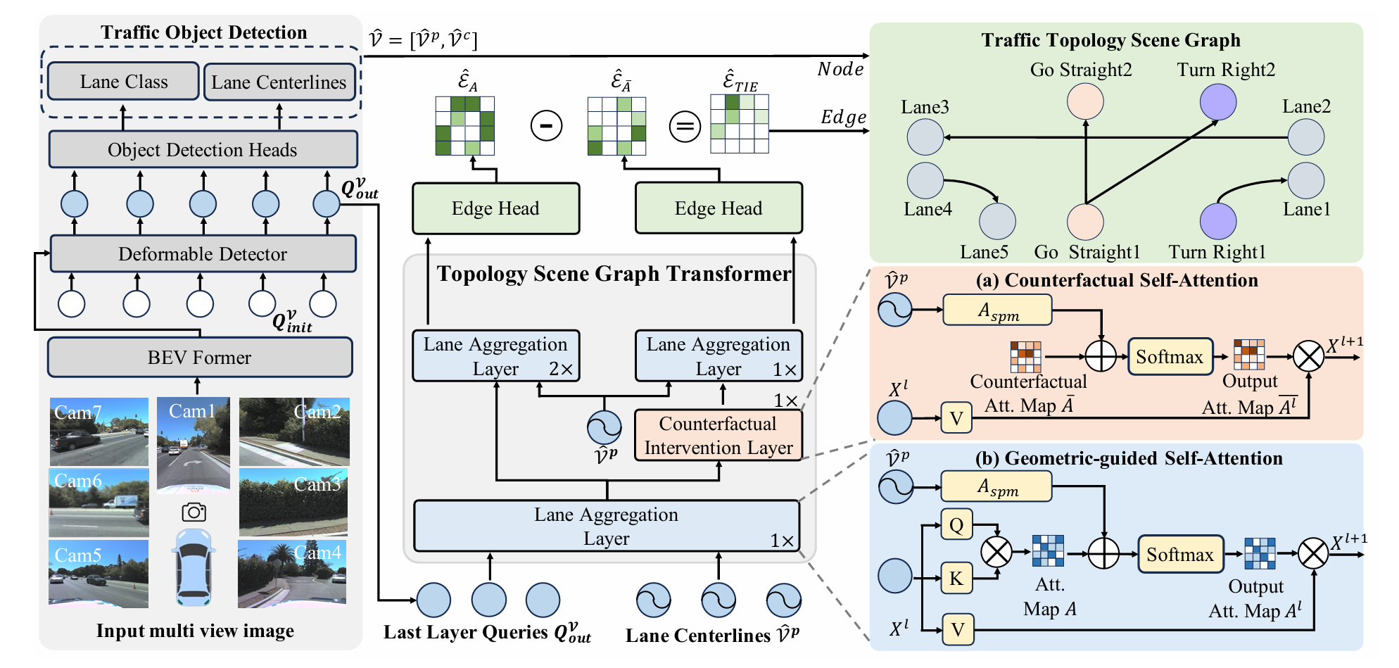
T2SG’s answer is a one-stage transformer called TopoFormer, with two new layers inside.
- Lane Aggregation Layer (LAL) — lanes gather information among themselves via self-attention, but a matrix built from endpoint distance is added as a bias to the attention so that “nearby lanes attend to each other more.” TopoLogic’s distance prior enters here not as a score but as an attention bias.
- Counterfactual Intervention Layer (CIL) — to judge whether a lane structure is actually reasonable, it uses the difference (causal effect) between the original and a deliberately broken counterfactual version of the learned attention as a training signal.
And the output is not a bare adjacency but a Traffic Topology Scene Graph (T2SG) — nodes are lanes, but instead of plain centerlines they carry 10 traffic semantic labels (go_straight, turn_left, no_u_turn, etc.), and edges are lane–lane connections in a directed graph. Where prior work treated “lanes as lanes, traffic as traffic” separately, T2SG models traffic rules (turn restrictions, etc.) and spatial connectivity in one graph.
Method
Pipeline overview
The big picture is the same BEV→DETR skeleton as the other posts in the series.
- Turn multi-view images into BEV features with BEVFormer.
- A Deformable DETR-style detector detects lane centerlines $\hat{\mathcal{V}}^p$ and classes $\hat{\mathcal{V}}^c$.
- Refine the detected lanes’ features by passing them through LAL → CIL in order.
- Predict lane–lane edges $\hat{\mathcal{E}}$ with the Edge Prediction Head.
Training is two-stage — pre-train the lane detector, then freeze it and train the T2SG task (LAL+CIL+edge head). (Just as TopoLogic was built on TopoNet, detection and relation learning are separated here.) Below we look at ① LAL and ② CIL with code and equations.
① Lane Aggregation Layer — distance as an attention bias
The core idea first. Treat lanes as nodes and gather global info via self-attention, but not plain attention — add a Spatial Proximity Matrix $A_\text{SPM}$, built from endpoint distance, to the attention score.
The distance matrix is essentially the same endpoint distance seen in TopoLogic — the distance between the end point of lane $i$ and the start point of lane $j$. Invert it (closer = larger) and normalize (paper Eq. 2).
The code is exactly this one line. Take the L2 distance of the centerline coordinate difference, form weights as $1/(d+\varepsilon)$, then normalize.
# projects/topoformer/models/dense_heads/spatial_proximity_head.py — forward()
dist = (center_A - center_B).pow(2)
dist = torch.sqrt(torch.sum(dist, dim=-1))[:, None, :, :]
dist_weights = 1 / (dist + 1e-2)
norm = torch.sum(dist_weights, dim=2, keepdim=True)
dist_weights = dist_weights / norm
Now feed this $A_\text{SPM}$ into self-attention. T2SG adds $A_\text{SPM}$ to the standard QK attention score — Geometry-guided Self-Attention (GSA) (paper Eq. 4).
Here the difference from TopoLogic sharpens. The same endpoint distance — TopoLogic used it as a topology score directly (distance → learnable function → 0–1 score → that is the adjacency), while T2SG uses it as an attention bias (distance → +α on the attention score → influences feature refinement). In the former, distance directly makes the final answer; in the latter, distance sets “which lanes mix more information.” So in T2SG a wrong distance doesn’t immediately become a wrong answer — the edge head judges once more after feature refinement.
🤔 (My take) what “add is best” implies. The ablation (paper Table 3) compares how to combine $A_\text{SPM}$ with attention, and Add (46.3) beats Hadamard (45.5) and Mul (45.7). The multiplicative variants kill attention entirely where the distance prior is near zero, whereas addition lays the prior on only as a bias, leaving the original attention alive. So “use distance only as a hint, let features make the final call” wins — which naturally sidesteps TopoLogic’s weakness of leaning too hard on distance and being sensitive to detection quality. (Reads as a lesson running through the whole series: injecting distance weakly as a bias is more robust than injecting it strongly as a score.)
② Counterfactual Intervention Layer — asking “does this structure make sense?”
This is where the paper is seen as most novel. CIL brings counterfactual intervention from causal inference into lane-structure reasoning.
The concern: attention does learn relations among lanes, but it’s hard to tell whether it captured a reasonable road structure or just memorized incidental patterns in the data. So CIL asks — “if there had been no learned interaction among lanes (counterfactual), how would the edge prediction differ?” That difference is “the causal effect that the learned road structure actually contributed.”
This is formalized as the Total Indirect Effect (TIE) — the factual prediction minus the counterfactual one (based on paper Eq. 6–7).
$\hat{\mathcal{E}}_A$ is the prediction with the learned attention $A$; $\hat{\mathcal{E}}_{\bar{A}}$ is the one with the counterfactual attention $\bar{A}$. At training time a loss is placed on this TIE, so the model directly optimizes “how much better do I predict relative to the counterfactual.” (At inference it just uses $\hat{\mathcal{E}}_A$ — TIE is a training device.)
So how is the counterfactual attention $\bar{A}$ made? The paper says it uses a zero matrix — zero out the learned attention to make the most unrealistic structure with “no interaction among lanes at all.” In the ablation, zero beats mean and random, and the authors explain that “a zero matrix represents a completely untrue road structure.”
⚠️ A gap between paper and code (again). The paper body describes the counterfactual as a zero matrix. But the official code’s
CounterfactualAttentionfills attention with random values on its default path —att = torch.randn(att_shape). The zero branch isn’t there (the# att = torch.randn_like(att)line above it is commented out, with no zero-fill line).
# projects/topoformer/utils/transformer.py — CounterfactualAttention.forward()
if self.use_counterfactual_att:
    # att = torch.randn_like(att)
    att = torch.randn(att_shape, device=v.device, dtype=v.dtype)   # ← random, not zero
else:
    att = torch.matmul(q, k) / np.sqrt(self.d_k)
The ablation clearly reports CIL-Zero above CIL-Random (46.3 vs 45.6), yet the public code’s default looks like the random side. When reproducing, it’s safest to check the config for which branch is on. (Recall TopoLogic’s “$\lambda\sigma$ vs a single $w$” gap — papers in this line diverge between body equations and released code quite a bit. The more so for the very selling point…)
CIL’s self-attention still receives $A_\text{SPM}$. That is, the counterfactual breaks only the learned QK attention, keeping the geometry prior (distance) identical on both sides — readable as “a physical fact like distance should hold even in the counterfactual.”
③ Loss
The loss is the sum of node and edge terms (paper Eq. 11–14).
The node loss is ordinary — focal on lane class, L1 on centerline coordinates. The point is that the edge loss is placed on $\hat{\mathcal{E}}_\text{TIE}$ (factual − counterfactual), not on $\hat{\mathcal{E}}_A$ — that’s the device that makes CIL learn.
OpenLane-V2 Benchmark & Results
Evaluation is the series’ usual OpenLane-V2, OLS. Subset_A numbers from paper Table 1.
| Method | $\text{DET}_l$ | $\text{TOP}_{ll}$ | $\text{TOP}_{lt}$ | OLS |
|---|---|---|---|---|
| TopoNet | 28.5 | 10.9 | 23.8 | 39.8 |
| TopoMLP | 28.3 | 21.6 | 26.9 | 44.1 |
| TopoLogic | 29.9 | 23.9 | 25.4 | 44.1 |
| TopoFormer | 34.7 | 24.1 | 29.5 | 46.3 |
- Detection jumps a lot. $\text{DET}_l$ 29.9 → 34.7, +4.8 over TopoLogic. Detection, stuck at 28–30 throughout the series, jumps once here, and a large share of the OLS rise comes from this (OLS includes detection as a direct term).
- $\text{TOP}_{ll}$ edges up only slightly. 23.9 → 24.1, +0.2 over TopoLogic. The lane–lane improvement itself is small. So this paper’s gain is less a dramatic lane–lane jump than a combination of detection + lane–traffic ($\text{TOP}_{lt}$ 25.4 → 29.5) + a bit of lane–lane.
- That sum lifts OLS 44.1 → 46.3 for the SOTA.
Ablation — how much each of LAL and CIL contributes
Paper Table 3 separates the two layers’ contributions.
- $A_\text{SPM}$ combination : none (45.4) < Hadamard (45.5) < Mul (45.7) < Add (46.3). Adding distance to attention is best.
- counterfactual type : none (44.9) < Mean (45.2) < Random (45.6) < Zero (46.3). The most unrealistic, zero, is best.
Both ablations have “weak prior (add) + strong counterfactual (zero)” winning. But as seen above, the table’s zero-is-best and the public code’s random default diverge — still bugs me… I’d have to run it myself.
Conclusion — relations inside attention, structure via counterfactual
To sum up, T2SG’s contribution is this.
Don’t classify lane–lane with a pairwise head; solve it inside self-attention among lanes, injecting the endpoint-distance prior not into the features but as a bias on the attention (LAL). And judge whether the learned road structure is reasonable via counterfactual intervention (TIE), using it for edge learning (CIL). The result lifts detection too and sets 46.3 OLS SOTA on OpenLane-V2 subset_A.
In the flow, T2SG’s place is clear. Where TopoNet used a graph, TopoMLP an MLP, and TopoLogic geometry to solve the relation, T2SG rewrites that geometry in the language of attention — putting distance in as a bias rather than a score, softening TopoLogic’s over-reliance on distance. Adding the counterfactual as a new axis is this paper’s own novelty.
What’s disappointing is that the real gain shows up in $\text{DET}$, not $\text{TOP}_{ll}$. The problem framing reads like “build topology without over-relying on detection,” so you’d expect TOP to be what rises — but the experiments end up proving the opposite.
Even so, the design — “solve the relation inside attention, and inject distance weakly as a bias” — together with bringing the counterfactual into lane structure, adds one more tool to this field. In the sparse lineage of lane topology reasoning, it’s a post that shows yet another angle.
Thanks for reading. If I’ve misunderstood anything, please let me know :)
comments