Splat2BEV — Reconstruction Matters: Learning Geometry-Aligned BEV Representation through 3D Gaussian Splatting
Paper review · Gaussian을 feature carrier로만 쓰지 말고, RGB로 재구성까지 시켜 geometry를 정렬한다.
각 figure의 출처는 하이퍼링크로 달아두었습니다 :)
+++ Gaussian Splatting for BEV Perception 섹션의 세 번째 글이다. GaussianBeV 글 결론에서 두 가지 문제점을 짚어뒀다 — (1) Gaussian 위치가 depth에 과의존한다, (2) Gaussian이 geometry를 옳게 잡았는지 RGB로 직접 검증받지 않는다. GaussianLSS가 첫째(depth)를 받았다면, Splat2BEV는 둘째를 정면으로 받는다. “Gaussian을 BEV feature 나르는 도구로만 쓰지 말고, RGB로 scene을 재구성하게 만들어 geometry를 검증·정렬하자.” 그래서 제목이 Reconstruction Matters다.
Reconstruction Matters: Learning Geometry-Aligned BEV Representation through 3D Gaussian Splatting
Authors : Yiren Lu, Xin Ye, Burhaneddin Yaman, Jingru Luo, Zhexiao Xiong, Liu Ren, Yu Yin (Bosch Research North America · Case Western Reserve University · Washington University in St. Louis)
Venue : arXiv 2026.03 (preprint) (ECCV 2026 format)
Paper Link : https://arxiv.org/abs/2603.19193
Code : 미공개
Introduction & Motivation
BEV를 black box로 학습한다는 것
앞 글에서 본 BEV 방법들은 — LSS든 BEVFormer든 GaussianBeV든, 심지어 GaussianLSS까지도 — 결국 한 방식으로 학습한다. image feature를 BEV 공간으로 옮기고, 그 BEV feature를 오직 downstream task loss로만 최적화한다. depth든 Gaussian이든 중간 표현은 task에 도움이 되는 방향으로 알아서 학습되길 기대할 뿐, 그게 실제 3D를 옳게 잡았는지는 explicit하게 모델링하지 않는다.
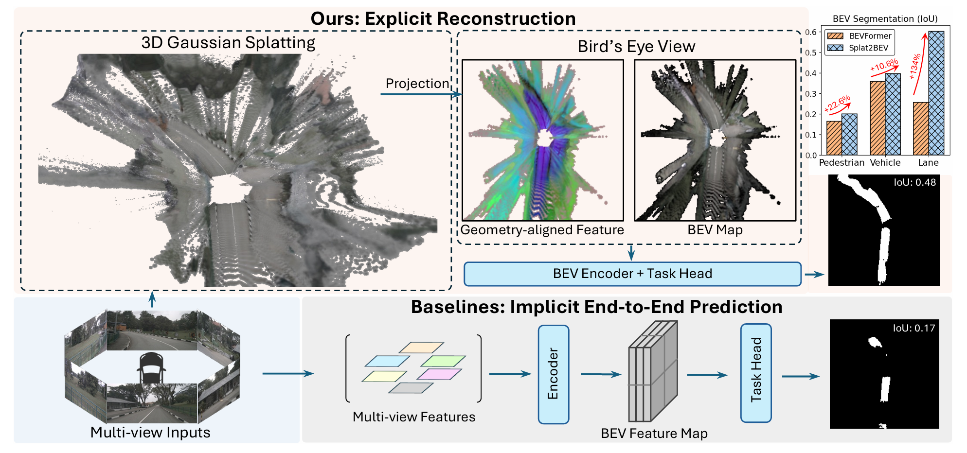
Splat2BEV의 문제 제기가 여기다. 이 end-to-end 방식은 perception 전체를 black box로 둔다. BEV feature가 좋은 segmentation을 내놓으면 그만이고, 그 안에 explicit한 3D geometry에 대한 이해가 들어있는지는 보장되지 않는다. 저자들은 이게 suboptimal하다고 본다. 기하를 명시적으로 잡지 못한 표현은 결국 한계가 있다는 것이다.
GaussianBeV 글 결론에서 짚은 두 번째 문제점이 정확히 이거였다. GaussianBeV·GaussianLSS는 Gaussian을 도입했지만, 그 Gaussian이 들고 있는 feature는 BEV task loss로만 간접 지도될 뿐 — Gaussian이 실제 3D를 옳게 잡았는지 맞춰보는 장치가 없었다. Splat2BEV는 이 둘을 정면으로 호명한다 (paper Section 2.2):
“GaussianLSS and GaussianBEV introduce 3D Gaussian Splatting as an intermediate representation… However, these two Gaussian Splatting–based methods treat the Gaussians merely as feature carriers rather than performing explicit 3D scene reconstruction.”
그래서 reconstruction을 시킨다
처방은 단순하고 직접적이다. Gaussian이 BEV feature를 나르기 전에, 먼저 RGB로 원본 이미지를 재구성하게 만든다. 재구성이 잘 된다는 건 Gaussian들이 3D 공간에 옳게 놓였다는 뜻이고, 그렇게 geometry가 정렬된 Gaussian에서 뽑은 feature를 BEV로 올리면 더 정확하다는 논리다.
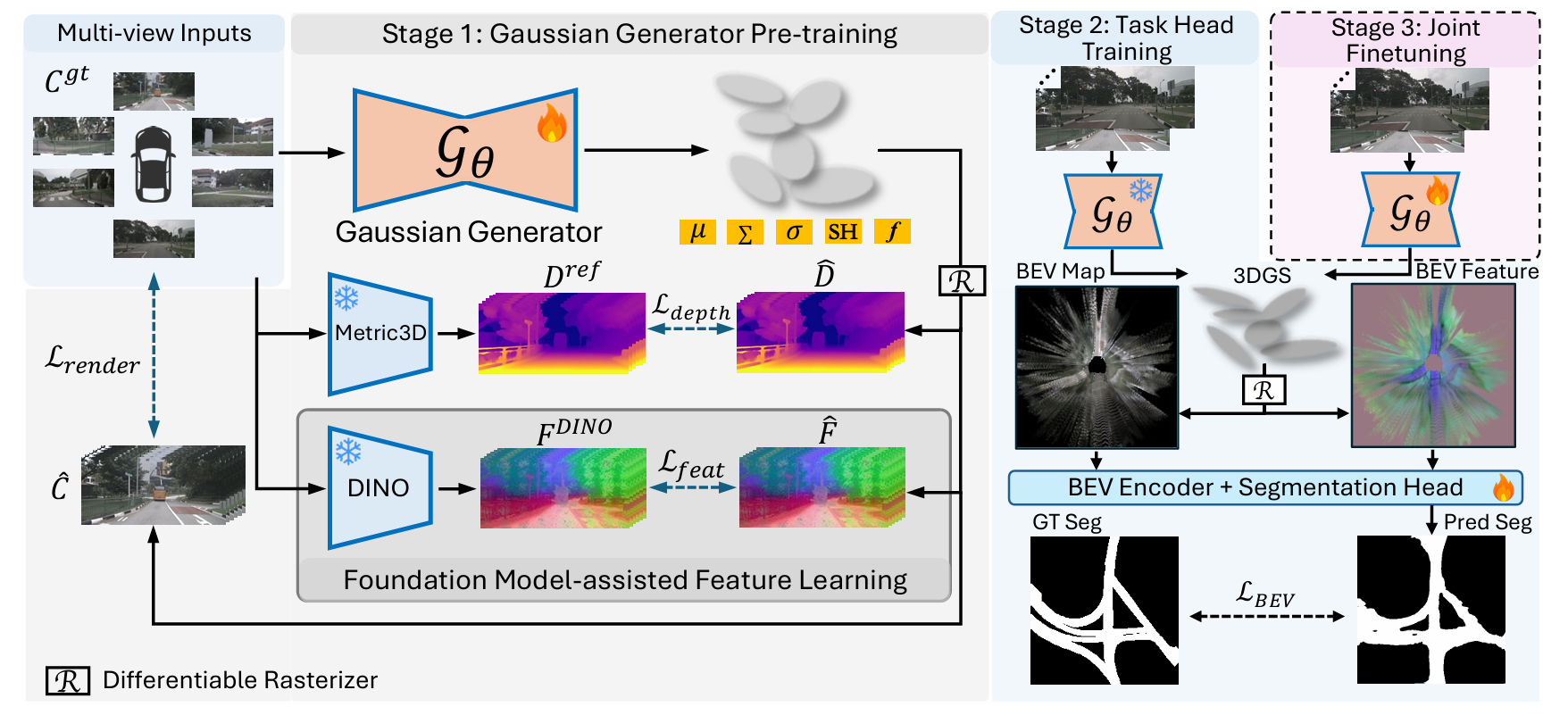
구체적으로 Splat2BEV는 Gaussian generator를 세 가지 supervision으로 pre-train한다.
- RGB rendering loss — Gaussian을 원본 view로 다시 렌더해 사진과 맞춘다(photometric MSE). geometry 검증의 핵심.
- depth supervision — Metric3Dv2가 준 metric depth로 Gaussian 위치를 grounding한다.
- feature distillation — DINOv2의 dense feature를 Gaussian feature에 distill해 semantic을 채운다.
즉 GaussianBeV가 “Gaussian을 task로만 학습”했다면, Splat2BEV는 “Gaussian을 RGB·depth·DINO로 먼저 빚어 놓고, 그 위에 task를 얹는다”. 같은 Gaussian splatting을 쓰되, 학습 신호를 task 바깥에서 끌어온다는 게 차이다.
Method
전체 파이프라인 — 3-stage
Splat2BEV는 한 번에 끝까지 학습하지 않는다. 세 단계로 나눈다.
- Stage 1 — Gaussian generator pre-training. 멀티뷰 이미지에서 Gaussian을 예측하고, RGB·depth·feature loss로 generator만 학습한다. 이 단계에서 geometry-aligned Gaussian이 만들어진다.
- Stage 2 — Task head training. generator를 얼리고, Gaussian을 BEV로 projection한 뒤 BEV encoder + task head를 학습한다.
- Stage 3 — Joint fine-tuning. 전부 풀어 end-to-end로 미세조정한다. task gradient가 generator까지 흘러간다.
epoch 배분은 10(Stage 1) + 10(Stage 2) + 20(Stage 3)이다. 핵심은 Stage 1 — task와 무관하게 “재구성이 되는 Gaussian”을 먼저 만들어 둔다는 것이다. 아래에서 ①Gaussian을 어떻게 뽑는지, ②Gaussian이 무엇을 드는지, ③Stage 1의 loss, ④BEV projection을 본다.
① Gaussian Generator — 멀티뷰에서 Gaussian을 뽑는 법
먼저 Gaussian을 어떻게 만드는지부터 보자. Splat2BEV의 generator는 scene별 최적화 없이 한 번의 forward로 Gaussian을 예측하는 feed-forward 방식이고(GaussianBeV·GaussianLSS와 같은 계열), 두 갈래의 branch를 쓴다 (paper Fig. 3).
- multi-view branch — UniMatch 기반으로, view들 사이 cost volume을 만들어 멀티뷰 기하 단서를 뽑는다. (서로 다른 view에서 같은 점이 어디 맺히는지를 cost volume이 잡아준다.)
- per-view branch — ViT-S로 각 view의 monocular feature를 뽑는다.
이 둘(cost volume + per-view feature)을 concat해 U-Net에 넣고, 거기서 view별 depth map과 Gaussian 속성들을 예측한다. 위치는 직접 regression하지 않는다 — depth map을 카메라 파라미터로 unproject해서 Gaussian의 mean position $\mu$를 얻고, 나머지 속성(covariance·opacity·SH·feature)은 separate head들이 따로 뽑는다.
📌 결국 pixel-aligned다. view별 depth map은 픽셀마다 depth 값 하나를 내고, 그걸 unproject하면 픽셀 하나당 3D 점(=Gaussian mean) 하나가 나온다. 즉 픽셀당 Gaussian 하나인 셈으로, GaussianBeV·GaussianLSS의 pixel-aligned 골격과 다르지 않다(PixelSplat·Splatter Image도 같은 구조다). 논문이 “pixel-aligned”라는 말을 쓰진 않지만, depth unproject로 위치를 잡는 한 그 결과는 자연히 pixel-aligned다. 차별점은 Gaussian을 어떻게 배치하느냐가 아니라, 그 Gaussian을 RGB·depth·DINO로 어떻게 학습시키느냐에 있다. 그리고 여러 view에서 나온 Gaussian들은 따로 병합·dedup하지 않고 전부 한 world 좌표계에 모아 그대로 렌더링한다. (중복은 opacity·rendering이 정리하도록 둔다).
② Gaussian이 가지는 값 — SH(RGB) + DINO feature
각 Gaussian $G_j$는 다섯 개의 값을 들고있다. (paper Eq. 7).
| 속성 | 기호 | 역할 |
|---|---|---|
| Position | $\mu_j$ | 3D 위치 (mean) |
| Covariance | $\Sigma_j$ | 3D 공분산 |
| Opacity | $\sigma_j$ | 불투명도 |
| Spherical Harmonics | $\text{SH}_j$ | view-dependent RGB (재구성용) |
| Feature | $f_j \in \mathbb{R}^C$ | DINO-distilled semantic feature |
앞 두 글과 결정적으로 다른 건 SH와 feature를 둘 다 든다는 점이다. GaussianBeV·GaussianLSS의 Gaussian은 색을 버리고 feature만 splat했다(그래서 RGB 검증이 불가능했다). Splat2BEV의 Gaussian은 SH로 RGB를 렌더해 geometry를 검증하고, feature로 BEV semantic을 나른다 — 한 Gaussian이 appearance와 semantic을 동시에 든다. 원조 3DGS에 가장 가까운 형태로 되돌아간 셈인데, 거기에 task feature를 하나 더 얹었다.
③ Stage 1 Loss — RGB·depth·feature 세 갈래
generator pre-training의 loss가 이 논문의 알맹이다 (paper Eq. 9).
$(\lambda_1, \lambda_2, \lambda_3) = (0.2, 0.8, 0.1)$이다. 셋을 하나씩 보면:
(1) RGB rendering loss. 3D-GS에서의 Reconstruction loss이다. Gaussian을 원본 카메라 view(Perspective-view)로 splat하여 얻어진 RGB값을 원본 이미지와 비교한다. 표준 3DGS alpha compositing으로 색을 누적하고(paper Eq. 2), GT 이미지와의 MSE를 건다 (paper Eq. 3).
이게 기존에 가지고 있었던 문제점을 메우는 핵심이다 — Gaussian이 RGB를 옳게 복원해야 한다는 직접 신호. 앞 두 글에는 없던 항이다.
(2) depth supervision. RGB만으로는 scale이 모호하니, depth를 따로 잡아준다. 여기서 비교하는 $\hat{D}$는 별도로 예측한 depth map이 아니라 Gaussian들을 ray 따라 alpha-blending해 렌더한 depth이고, 이걸 Metric3Dv2가 준 reference depth $D^\text{ref}$에 맞춘다. L1과 SILog 두 항을 쓴다 (paper Eq. 4–5).
$\delta_i(p) = \log \hat{D}_i(p) - \log D_i^\text{ref}(p)$로, L1은 절대 depth를, SILog는 scale-invariant한 상대 구조를 맞춘다(전체적으로 일정하게 어긋난 scale 오차에는 둔감하고, 픽셀 간 상대 깊이 패턴을 본다). depth가 잡히면 Gaussian의 $\mu_j$가 실제 3D 표면에 붙는다.
(3) feature distillation. 렌더한 feature를 DINOv2의 dense feature에 맞춘다 — cosine similarity loss다 (paper Eq. 8).
즉 geometry는 RGB·depth로, semantic은 DINO로 잡는다. RGB rendering이 feature와 같은 alpha compositing을 공유하므로(색 $\mathbf{c}$ 자리에 feature $\mathbf{f}$를 넣으면 feature 렌더가 된다), 둘이 같은 Gaussian 위에서 일관되게 학습된다.
🤔 (사견) reconstruction은 도구지 목적이 아니다. 이 논문이 RGB로 재구성을 시키는 건 예쁜 novel view를 만들려는 게 아니라, “reconstruction이 적당히 되면 geometry 또한 어느정도 맞은 것”이라는 proxy를 쓰려는 것이다. 그런데 한 가지 짚을 게 있다. reconstruction은 training view에서만 검증된다. 원본 카메라 pose로 다시 렌더해 맞추지, 학습에 안 쓴 novel pose로 일반화되는지는 안 본다. training view 재구성이 잘 된다고 그 Gaussian이 진짜 3D를 잡았다는 보장은 약하다 — overfit된 Gaussian도 자기가 본 view는 잘 복원하니까. depth supervision(Metric3Dv2)이 이걸 보완하긴 하는데, 결국 “reconstruction matters”라는 제목의 무게는 RGB loss 단독보다 RGB+depth 조합에서 온다고 보는 게 맞겠다. 또한 semantic feature를 왜 같이 reconstruction에 쓰는지는 아직 잘 모르겠는데.. 더 읽어보자.
④ BEV Projection — orthographic으로 splat한다
Stage 1에서 깎은 Gaussian을 BEV로 올린다. 핵심은 orthographic projection이다 — perspective가 아니라 위에서 수직으로 내려다보는 투영이어야 BEV 평면이 된다(GaussianBeV의 orthographic splatting을 수식으로 구체화한 셈).
먼저 Gaussian의 mean을 BEV 평면 좌표로 투영한다. perspective projection matrix 대신 orthographic matrix $M_\text{ortho}$를 쓴다 — 핵심은 depth 항이 빠진다는 것이다(paper Eq. 10–11).
perspective와의 진짜 차이는 depth로 나누느냐다. perspective는 $u = f_x X/Z$처럼 $Z$로 나눠서(perspective divide) 멀수록 작게 모이는 원근이 생긴다. orthographic은 $u = f_x X + c_x$로 나눗셈이 없다 — $M_\text{ortho}$의 마지막 행이 $[0\,0\,0\,1]$이라 동차좌표 $w$가 1로 고정되고, $Z$항(세 번째 열)도 0이라 $(X,Y)$만으로 $u,v$가 정해진다. 그래서 멀든 가깝든 같은 $(X,Y)$면 BEV의 같은 칸에 떨어진다 — 원근 왜곡이 없다. 동시에 $Z$를 버린다는 건 곧 높이를 눌러 3D를 top-down 평면으로 납작하게 만든다는 뜻이고, 이게 BEV의 본질이다.
covariance도 같이 2D로 내려야 한다. Gaussian은 점이 아니라 퍼짐을 가진 타원체라, 위치만 투영하면 안 되고 그 모양(공분산)도 평면에서 어떻게 보일지 변환해야 한다. 핵심은 — 투영이 비선형이면 Gaussian을 그대로 투영해도 Gaussian이 안 되므로, 투영 함수를 그 점 근처에서 1차 선형 근사(Jacobian $J$)한 뒤 그 선형변환으로 공분산을 옮기는 것이다(EWA splatting의 표준). 선형변환 $J$ 아래에서 공분산은 $J \Sigma J^\top$로 변하므로 (paper Eq. 12–13):
여기서 orthographic이라 한 가지가 단순해진다 — $J_\text{ortho}$가 상수($f_x, f_y$)로, Gaussian의 위치·depth에 안 변한다. perspective였다면 Jacobian에 $1/Z$ 같은 항이 끼어 Gaussian마다 달라지는데(그래서 멀리 있는 게 작게 찌그러진다), orthographic은 그 의존이 없어 모든 Gaussian이 같은 $J$로 눌린다. 위치 투영이 단순해진 것과 같은 이유다.
이렇게 평면에 내린 2D Gaussian들을 rasterize한다. (gsplat 라이브러리 사용) -> 색 자리에 feature를 넣어(앞서 본 그 alpha compositing) BEV feature map을 rendering한다. 실험 세팅은 200×200 격자, 100m 범위, BEV 카메라 높이는 +3m다(z축 offset). 그 위에 BEV encoder와 segmentation head를 얹는다.
task loss는 평범하다 — focal + centerness(L2) + offset(L1) (paper Eq. 14). Stage 2에서는 generator를 얼린 채 이 head만 학습하고, Stage 3에서 전부 풀어 같이 joint fine-tuning한다.
📌 Stage 1만으로도 꽤 된다. ablation(paper Table 6)이 흥미롭다 — generator를 얼린 채(joint fine-tuning 없이) BEV head만 학습해도 lane IoU 49.2가 나온다. 즉 task gradient가 generator에 닿기 전, RGB·depth·DINO만으로 빚은 Gaussian feature가 이미 BEV에 쓸 만하다는 뜻이다. 이게 이 논문의 thesis를 가장 직접 뒷받침하는 숫자다 — geometry-aligned 표현은 task supervision 없이도 일찍 만들어진다.
🤔 (사견) RGB로 깎은 covariance는 PV 기준인데, BEV에선 점처럼 깔릴 위험이 있다.
한 가지 걸리는 게 있다. Stage 1의 covariance는 결국 RGB rendering loss로 학습되는데, 그 loss는 원본 카메라 view(PV)에서 사진을 선명하게 맞추는 방향이다. photometric loss로 빡세게 학습된 3DGS는 sharp한 detail을 잡으려 Gaussian이 잘게 쪼개지는 경향이 매우 크다. 즉 covariance가 PV에서 선명한 쪽으로 최적화된다. 하지만 BEV splat은 orthographic이라 거리로 안 줄어드니, $\Sigma_\text{3D}$가 실제로 작으면 그게 BEV 평면에 그대로 작은 점처럼 찍힐 것이다. 다시 말해 PV용으로 작게 깎여진 Gaussian이 BEV에선 sparse한 점들로 깔려 feature map에 구멍이 날 수 있다는 얘기다. lane처럼 얇은 구조가 가장 먼저 깨질 곳일텐데…
논문에서 이 둘을 완화하는 장치는 있다 — depth supervision이 $\Sigma$를 3D 표면에 grounding하고, Stage 3 joint fine-tuning이 BEV task loss로 generator를 다시 민다(ablation에서 w/o 3-stage일 때 lane이 60.2 → 56.7로 떨어지는 게, 이 보정이 실제로 작동한다는 간접 정황이다). 다만 이건 말 그대로 완화지 근본 해결은 아닐 것 같다. depth는 Gaussian을 표면에 붙이는 제약이지 BEV에서 적절히 퍼지게 하는 제약이 아니고, joint FT도 PV rendering loss와 BEV task loss가 covariance를 서로 반대로 당기는 줄다리기이다. 즉 RGB를 잘 맞추려는 압력(작게)과 BEV를 잘 덮으려는 압력(크게)이 충돌할 것이다. “RGB 재구성으로 깎은 geometry”라는 이 논문의 핵심 전제 자체가, BEV splat의 입장에선 애초에 다른 목적함수로 최적화된 Gaussian을 빌려 쓰는 구조라, 이 gradient collision 자체가 trick 몇 개로 사라지진 않을 것이다. (논문이 Stage 1 후 BEV에서의 Gaussian density나 빈 칸을 직접 시각화·측정하진 않아, 이게 실제로 얼마나 문제였는지는 표만으론 알 수 없다.)
nuScenes & Argoverse Benchmark & Results
평가는 nuScenes·Argoverse BEV segmentation, metric은 IoU다.
Vehicle IoU (nuScenes):
| Method | 224×480 | 448×800 |
|---|---|---|
| GaussianLSS | 38.3 | 40.6 |
| PointBeV | 38.7 | 42.1 |
| Splat2BEV | 39.6 | 42.7 |
클래스별 (nuScenes, 224×480):
| Class | PointBeV | GaussianLSS | Splat2BEV |
|---|---|---|---|
| Pedestrian | 18.5 | 18.0 | 20.1 |
| Lane | 49.6 | — | 60.2 |
- vehicle은 소폭 앞선다. PointBeV 대비 +0.9(224×480), +0.6(448×800). GaussianLSS(38.3)도 넘는다.
- lane에서 격차가 크다. 49.6 → 60.2로 +21.4%. lane은 얇고 길어 정확한 geometry가 특히 중요한 클래스인데, reconstruction으로 기하를 정렬한 효과가 여기서 가장 크게 드러난다. (이 논문이 자기 강점을 가장 잘 보여주는 숫자가 lane이다.)
- multi-class mIoU도 nuScenes 34.4, Argoverse 24.4로 SOTA를 찍는다.
Ablation — 무엇이 효과를 냈나
paper Table 7이 모듈을 떼어 본다(nuScenes 224×480, vehicle/ped/lane).
- full : 39.6 / 20.1 / 60.2
- w/o 3-stage : 38.3 / 18.1 / 56.7 — 3단계 학습을 빼면(한 번에 학습) lane이 60.2 → 56.7로 크게 떨어진다. pre-train으로 geometry를 먼저 잡는 게 lane에 결정적이다.
- w/o DINO : 37.9 / 17.6 / 56.3 — DINO distillation을 빼면 전 클래스가 떨어진다. semantic 보강이 빠지면 reconstruction만으로는 부족하다는 것.
두 ablation 다 “reconstruction(3-stage) + semantic(DINO)”이 같이 있어야 best다. geometry만으로도, semantic만으로도 부족하고 둘을 합쳐야 한다는 그림이다.
Conclusion — Gaussian에 재구성을 시킨다
정리하면, Splat2BEV의 기여는 이렇다.
BEV를 task loss만으로 학습하면 geometry가 black box로 남는다. 그러니 Gaussian을 BEV feature를 lifting하는 도구로만 쓰지 말고, RGB rendering·depth·DINO distillation으로 먼저 scene을 재구성하도록 pre-train해 geometry-aligned 표현을 만든 뒤 BEV로 올려라.
GaussianBeV가 “Gaussian으로 BEV를 만들 수 있다”를 보이고 GaussianLSS가 “그 Gaussian이 depth 불확실성을 담을 수 있다”를 보탰다면, Splat2BEV는 앞 글에서 짚은 두 번째 문제점 — Gaussian이 geometry를 직접 검증받지 않는다 — 을 정면으로 메운다. RGB로 재구성을 시켜 “이 Gaussian이 3D를 옳게 잡았나”를 직접 묻는다.
개인적으로 솔직한 감상은… 접근(reconstruction을 BEV에 끌어온다)은 좋은데, 그걸 푸는 방식엔 novelty가 거의 없다. 뜯어보면 대부분이 이미 있는 연구고, 그것들의 조합이다. feed-forward GS, BEV splat, depth supervision, semantic feature — 어느 하나 새로 만든 게 아니라 다 incremental하게 가져다 쓴 것이고, 심지어 geometry는 Metric3Dv2, semantic은 DINOv2로 foundation model의 distillation까지 받아가며 채운다. 방법론만 보면 “있는 걸 잘 엮었다” 이상을 말하기 어렵다.
그럼에도 이 연구가 가지는 의미는 분명있다. Stage 3 joint fine-tuning에서 성능이 오른다는 것 — 이게 “PV에서 맞춘 geometry가 BEV geometry에도 실제로 효과가 있다”를 보여준 지점이다. 앞서 사견으로 짚었듯 PV에서 RGB용으로 깎은 Gaussian이 BEV에 그대로 좋으리란 보장은 없는데, joint FT로 그 둘을 이어붙였을 때 실제로 숫자가 오른다면, PV reconstruction이라는 신호가 BEV 표현에 transferring이 가능하다는 증거가 된다. 방법 하나하나는 새롭지 않아도, 이 한 가지를 실험만으로 인정할 만하다.
읽어주셔서 감사합니다. 혹시 제가 잘못 이해한 부분이 있다면 언제든 알려주세요 :)
Figure sources are linked inline :)
+++ Third post in the Gaussian Splatting for BEV Perception section. The GaussianBeV post flagged two problems in its conclusion — (1) Gaussian position over-relies on depth, (2) whether a Gaussian got the geometry right is never directly verified with RGB. If GaussianLSS took on the first (depth), Splat2BEV takes on the second head-on. “Don’t use the Gaussian merely as a carrier of BEV features; make it reconstruct the scene with RGB to verify and align the geometry.” Hence the title Reconstruction Matters.
Reconstruction Matters: Learning Geometry-Aligned BEV Representation through 3D Gaussian Splatting
Authors : Yiren Lu, Xin Ye, Burhaneddin Yaman, Jingru Luo, Zhexiao Xiong, Liu Ren, Yu Yin (Bosch Research North America · Case Western Reserve University · Washington University in St. Louis)
Venue : arXiv 2026.03 (preprint)
Paper Link : https://arxiv.org/abs/2603.19193
Code : not released
Introduction & Motivation
What it means to learn BEV as a black box
The BEV methods seen in the previous two posts — LSS, BEVFormer, GaussianBeV — all train in one way in the end. They move image features into the BEV space and optimize that BEV feature solely through downstream task loss (segmentation, etc.). Whether the intermediate representation is depth or Gaussians, it’s just expected to learn in whatever direction helps the task; whether it actually got the 3D right is never directly asked.
Splat2BEV’s complaint is here. This end-to-end formulation leaves the whole perception as a black box. If the BEV feature yields good segmentation, that’s enough; there’s no guarantee it contains an explicit 3D geometric understanding. The authors call this suboptimal — a representation that fails to capture geometry explicitly is ultimately limited.
That’s exactly the second problem flagged in the GaussianBeV post’s conclusion. GaussianBeV·GaussianLSS introduced Gaussians, but the features those Gaussians carry are only indirectly supervised by the BEV task loss — with no mechanism to check, via RGB, whether the Gaussian got the 3D right. Splat2BEV calls the two out by name (paper §2.2):
“GaussianLSS and GaussianBEV introduce 3D Gaussian Splatting as an intermediate representation… However, these two Gaussian Splatting–based methods treat the Gaussians merely as feature carriers rather than performing explicit 3D scene reconstruction.”
So it makes them reconstruct
The prescription is simple and direct. Before the Gaussian carries a BEV feature, make it reconstruct the original image with RGB. Good reconstruction means the Gaussians sit correctly in 3D space, and features pulled from such geometry-aligned Gaussians, lifted to BEV, should be more accurate.
Concretely, Splat2BEV pre-trains the Gaussian generator with three supervisions.
- RGB rendering loss — render the Gaussians back to the original views and match the photos (photometric MSE). The core of geometric verification.
- depth supervision — ground Gaussian positions with metric depth from Metric3Dv2.
- feature distillation — distill DINOv2’s dense features into the Gaussian features to fill in semantics.
So where GaussianBeV “learned Gaussians by task alone,” Splat2BEV “shapes the Gaussians first with RGB·depth·DINO, then mounts the task on top.” Same Gaussian splatting, but the difference is that it draws training signal from outside the task.
Method
Pipeline — 3 stages
Splat2BEV doesn’t train end-to-end in one shot. It splits into three stages.
- Stage 1 — Gaussian generator pre-training. Predict Gaussians from multi-view images and train only the generator with RGB·depth·feature losses. This is where geometry-aligned Gaussians are made.
- Stage 2 — Task head training. Freeze the generator, project the Gaussians to BEV, and train the BEV encoder + task head.
- Stage 3 — Joint fine-tuning. Unfreeze everything and fine-tune end-to-end; task gradients flow back to the generator.
The epoch split is 10 (Stage 1) + 10 (Stage 2) + 20 (Stage 3). The key is Stage 1 — make “Gaussians that reconstruct” first, independent of the task. Below we look at ① how the Gaussians are produced, ② what a Gaussian carries, ③ the Stage 1 loss, ④ the BEV projection.
① Gaussian Generator — producing Gaussians from multi-view
First, how the Gaussians are made. Splat2BEV’s generator is feed-forward — predicting Gaussians in a single forward pass without per-scene optimization (the same family as GaussianBeV·GaussianLSS) — and uses two branches (paper Fig. 3).
- multi-view branch — based on UniMatch, it builds cost volumes across views to extract multi-view geometric cues. (The cost volume captures where the same point lands across different views.)
- per-view branch — a ViT-S extracts each view’s monocular features.
The two (cost volume + per-view features) are concatenated into a U-Net, which predicts a per-view depth map and the Gaussian attributes. Position isn’t regressed directly — the depth map is unprojected with camera parameters to get the Gaussian mean $\mu$, and the rest (covariance·opacity·SH·feature) come from separate heads.
📌 It’s pixel-aligned in the end. The per-view depth map emits one depth value per pixel, and unprojecting it yields one 3D point (= Gaussian mean) per pixel. So it’s one Gaussian per pixel — no different from the pixel-aligned skeleton of GaussianBeV·GaussianLSS (PixelSplat·Splatter Image share the same structure). The paper doesn’t use the word “pixel-aligned,” but as long as positions are set by depth unprojection, the result is naturally pixel-aligned. The distinction isn’t in how the Gaussians are arranged but in how they’re trained — with RGB·depth·DINO. And Gaussians from multiple views aren’t merged or deduplicated — they’re all gathered in one world frame and rendered as-is (overlaps left for opacity·rendering to sort out).
② What a Gaussian carries — SH (RGB) + DINO feature
Each Gaussian $G_j$ carries five things (paper Eq. 7).
| Attribute | Symbol | Role |
|---|---|---|
| Position | $\mu_j$ | 3D position (mean) |
| Covariance | $\Sigma_j$ | 3D covariance |
| Opacity | $\sigma_j$ | opacity |
| Spherical Harmonics | $\text{SH}_j$ | view-dependent RGB (for reconstruction) |
| Feature | $f_j \in \mathbb{R}^C$ | DINO-distilled semantic |
The decisive difference from the previous two posts is that it carries both SH and feature. GaussianBeV·GaussianLSS dropped color and splatted only features (which is why RGB verification was impossible). Splat2BEV’s Gaussian renders RGB via SH to verify geometry, and carries features to ferry BEV semantics — one Gaussian holds appearance and semantics at once. It’s a return to the form closest to vanilla 3DGS, with one task feature added on top.
③ Stage 1 Loss — three paths: RGB·depth·feature
The generator pre-training loss is the heart of this paper (paper Eq. 9).
with $(\lambda_1, \lambda_2, \lambda_3) = (0.2, 0.8, 0.1)$. One at a time:
(1) RGB rendering loss. Splat the Gaussians back to the original camera view and match the photo. Accumulate color with standard 3DGS alpha compositing (paper Eq. 2) and apply an MSE against the GT image (paper Eq. 3).
This is the core that fills the “second problem” — a direct signal that the Gaussian must reconstruct RGB correctly. A term the previous two posts didn’t have.
(2) depth supervision. RGB alone leaves scale ambiguous, so depth is grounded separately. The $\hat{D}$ compared here isn’t a separately predicted depth map but a depth rendered by alpha-blending the Gaussians along the ray, matched against the reference depth $D^\text{ref}$ from Metric3Dv2. Two terms, L1 and SILog (paper Eq. 4–5).
with $\delta_i(p) = \log \hat{D}_i(p) - \log D_i^\text{ref}(p)$. L1 matches absolute depth; SILog matches the scale-invariant relative structure (insensitive to a uniform scale offset, looking instead at the relative depth pattern across pixels). Once depth is fixed, the Gaussian’s $\mu_j$ sticks to the actual 3D surface.
(3) feature distillation. Match the rendered feature to DINOv2’s dense features — a cosine similarity loss (paper Eq. 8).
So geometry comes from RGB·depth, semantics from DINO. Since RGB rendering shares the same alpha compositing as the feature (substitute feature $\mathbf{f}$ for color $\mathbf{c}$ and you get the feature render), the two are learned consistently on the same Gaussian.
🤔 (My take) reconstruction is a tool, not the goal. The paper makes it reconstruct with RGB not to produce pretty novel views but to use the proxy “if it reconstructs, the geometry is right.” But one thing to note — the reconstruction is verified only on training views. It re-renders to the original camera poses and matches; whether it generalizes to novel poses unseen in training isn’t checked. Good reconstruction on training views is weak evidence that the Gaussian truly captured 3D — an overfit Gaussian also reconstructs the views it saw. The depth supervision (Metric3Dv2) does compensate, but in the end the weight behind the title “reconstruction matters” comes more from RGB+depth together than RGB loss alone.
④ BEV Projection — splat orthographically
Lift the Gaussians shaped in Stage 1 to BEV. The key is orthographic projection — a straight-down projection, not perspective, is what makes a BEV plane (concretizing GaussianBeV’s orthographic splatting into equations).
First project the Gaussian mean to BEV-plane coordinates. Instead of a perspective projection matrix, use an orthographic matrix $M_\text{ortho}$ — the key being that the depth term drops out (paper Eq. 10–11).
The zero third column is the difference from perspective — $G_Z$ (depth) doesn’t affect $u, v$, so the same $(X, Y)$ lands in the same BEV cell whether far or near. That’s why it yields a perspective-free planar map.
The covariance must be dropped to 2D too. The 3D covariance $\Sigma_\text{3D}$ is transformed by the orthographic projection’s Jacobian $J_\text{ortho}$ (paper Eq. 12–13).
These 2D Gaussians dropped onto the plane are rasterized with gsplat — substituting feature for color (the same alpha compositing) renders the BEV feature map. The experimental setting is a 200×200 grid, 100m range, BEV camera height +3m (z-axis offset). A BEV encoder and segmentation head go on top.
The task loss is ordinary — focal + centerness (L2) + offset (L1) (paper Eq. 14). Stage 2 trains only this head with the generator frozen; Stage 3 unfreezes everything for joint fine-tuning.
📌 Stage 1 alone already gets you far. The ablation (paper Table 6) is telling — with the generator frozen (no joint fine-tuning), training only the BEV head still yields lane IoU 49.2. That is, before any task gradient reaches the generator, Gaussian features shaped by RGB·depth·DINO alone are already usable for BEV. This is the number that most directly supports the paper’s thesis — a geometry-aligned representation is formed early, without task supervision.
🤔 (My take) covariance shaped by RGB is PV-centric, and risks landing as dots in BEV. One thing nags. Stage 1’s covariance is ultimately learned by the RGB rendering loss, which aims to sharpen the photo in the original camera view (PV). A 3DGS trained hard by photometric loss tends to split Gaussians small to chase sharp detail — i.e. the covariance is optimized to be crisp in PV. But BEV splatting is orthographic, so it doesn’t shrink with distance; if $\Sigma_\text{3D}$ is genuinely small, it stamps onto the BEV plane as a small dot. Gaussians shaped small for PV can scatter as sparse dots in BEV, leaving holes in the feature map — and thin structures like lanes would break first.
The paper does have mitigations — depth supervision grounds $\Sigma$ on the 3D surface, and Stage 3 joint fine-tuning pushes the generator with the BEV task loss (the lane drop 60.2 → 56.7 in the w/o-3-stage ablation is indirect evidence that this correction actually works). But this is mitigation, not a fundamental fix. Depth constrains Gaussians to stick to surfaces, not to spread appropriately in BEV; and joint FT is a tug-of-war where the PV rendering loss and the BEV task loss pull the covariance in opposite directions — the pressure to match RGB (small) clashes with the pressure to cover BEV (large). The paper’s core premise — “geometry shaped by RGB reconstruction” — means BEV splatting is borrowing Gaussians optimized for a different objective in the first place, so this tension won’t vanish with a few tricks. (The paper doesn’t visualize or measure the post-Stage-1 Gaussian density or holes in BEV, so how much of a problem this actually was can’t be told from the tables alone.)
nuScenes & Argoverse Benchmark & Results
Evaluation is BEV segmentation on nuScenes and Argoverse, metric IoU.
Vehicle IoU (nuScenes):
| Method | 224×480 | 448×800 |
|---|---|---|
| GaussianLSS | 38.3 | 40.6 |
| PointBeV | 38.7 | 42.1 |
| Splat2BEV | 39.6 | 42.7 |
Per class (nuScenes, 224×480):
| Class | PointBeV | GaussianLSS | Splat2BEV |
|---|---|---|---|
| Pedestrian | 18.5 | 18.0 | 20.1 |
| Lane | 49.6 | — | 60.2 |
- Vehicle edges ahead. +0.9 over PointBeV (224×480), +0.6 (448×800). It also passes GaussianLSS (38.3).
- The gap is large on lane. 49.6 → 60.2, +21.4%. Lane is thin and long, a class where precise geometry matters most, and the effect of aligning geometry via reconstruction shows up biggest here. (Lane is the number that best showcases this paper’s strength.)
- Multi-class mIoU also sets SOTA — 34.4 on nuScenes, 24.4 on Argoverse.
Ablation — what drove the gains
Paper Table 7 peels off the modules (nuScenes 224×480, vehicle/ped/lane).
- full : 39.6 / 20.1 / 60.2
- w/o 3-stage : 38.3 / 18.1 / 56.7 — drop the 3-stage scheme (train in one go) and lane falls 60.2 → 56.7. Grabbing geometry first via pre-training is decisive for lane.
- w/o DINO : 37.9 / 17.6 / 56.3 — drop DINO distillation and every class falls. Without the semantic boost, reconstruction alone isn’t enough.
Both ablations need “reconstruction (3-stage) + semantics (DINO)” together for the best. Geometry alone isn’t enough, semantics alone isn’t enough — you need both.
Conclusion — make the Gaussian reconstruct
To sum up, Splat2BEV’s contribution is this.
Learning BEV by task loss alone leaves geometry a black box. So don’t use the Gaussian merely as a carrier of BEV features — pre-train it to reconstruct the scene with RGB rendering·depth·DINO distillation, building a geometry-aligned representation before lifting to BEV. The result is SOTA on nuScenes·Argoverse, especially +21.4% on lane.
Splat2BEV’s place in the series is clear. GaussianBeV showed “you can build BEV with Gaussians” and GaussianLSS added “those Gaussians can carry depth uncertainty”; Splat2BEV fills the second problem flagged in the earlier post — that the Gaussian’s geometry is never directly verified — head-on. It makes them reconstruct with RGB and asks directly, “did this Gaussian get the 3D right?”
My honest take: the approach (bringing reconstruction into BEV) is good, but there’s almost no novelty in how it’s solved. Pick it apart and it’s nearly all off-the-shelf parts combined. Feed-forward GS, BEV splat, depth supervision, semantic features — none newly invented, all pulled in incrementally; and it even fills geometry with Metric3Dv2 and semantics with DINOv2, leaning on foundation-model distillation. On method alone it’s hard to say more than “well assembled from what’s already there.”
Still, there’s something to credit. Performance rises under Stage 3 joint fine-tuning — and that’s the point where it shows “geometry fitted in PV actually carries over to BEV geometry.” As flagged in the earlier aside, there’s no guarantee that Gaussians shaped for PV are good as-is in BEV; but if joining the two via joint FT actually moves the numbers up, that’s evidence the PV-reconstruction signal transfers into the BEV representation. No single component is new, but demonstrating empirically that “geometry shaped by RGB reconstruction can be transferred to BEV” is worth acknowledging.
Thanks for reading. If I’ve misunderstood anything, please let me know :)
comments