GaussianBeV — 3D Gaussian Representation Meets Perception Models for BeV Segmentation
Paper review · turning every pixel into an oriented 3D Gaussian, then splatting them into the BEV plane.
각 figure의 출처는 하이퍼링크로 달아두었습니다 :)
+++ Gaussian Splatting for BEV Perception 섹션의 첫 번째 글이다. 이 시리즈는 “BEV feature를 어떻게 만들 것인가”라는 오래된 질문에, 최근의 3D Gaussian Splatting이 내놓은 대답들을 따라간다. 출발점은 GaussianBeV다 — scene reconstruction을 위한 도구였던 3DGS를, scene별 최적화 없이 한 번의 forward로 image→BEV 변환에 끼워 넣은 첫 시도. “이미지의 한 픽셀을 3D 공간에 떠 있는 작은 타원체(Gaussian) 하나로 보고, 그것들을 위에서 내려다보며 뭉개면(splat) BEV feature가 된다”는 발상이다.
GaussianBeV: 3D Gaussian Representation meets Perception Models for BeV Segmentation
Authors : Florian Chabot, Nicolas Granger, Guillaume Lapouge (CEA-List, Université Paris-Saclay · CEA–Valeo joint lab)
Venue : WACV 2025
Paper Link : https://arxiv.org/abs/2407.14108
Code : 미공개 (공식 구현 없음)
Introduction & Motivation
image → BEV, 그 변환을 누가 어떻게 해왔나
자율주행 인지의 거의 모든 파이프라인은 한 지점에서 같은 고민을 만난다 — 여러 대의 카메라가 찍은 perspective 이미지를, 위에서 내려다본 하나의 BEV(Bird’s-eye View) 평면으로 어떻게 옮길 것인가. detection이든 segmentation이든, 심지어 E2E Planning까지도, 그 위에 얹히는 task들은 대개 이 BEV feature가 얼마나 좋은지에 운명이 걸려 있다.
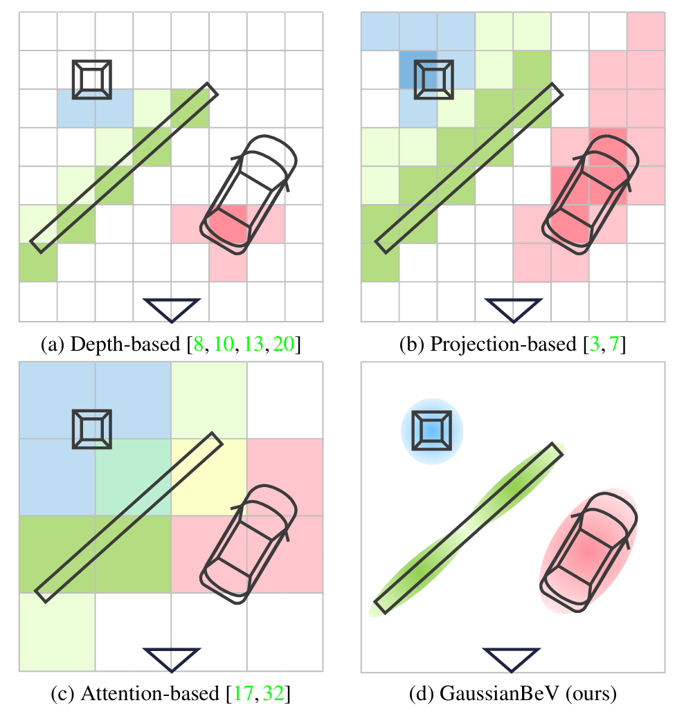
그 변환을 푸는 방식은 크게 두 갈래로 굳어져 있었다.
- Lift-Splat-Shoot (LSS) 계열 — “픽셀을 들어 올린다(lift)”. 각 픽셀마다 depth 분포를 예측해, 그 분포를 따라 feature를 카메라 ray 위로 흩뿌린 뒤(lift), BEV 격자에 떨어뜨려 모은다(splat). depth가 명시적이라 기하는 또렷하지만, depth를 이산적인 bin들의 분포로만 다뤄 표현이 거칠다.
- BEVFormer·Simple-BEV 계열 — “BEV에서 거꾸로 본다”. BEV 격자의 각 칸(query)을 정해두고, 그 칸이 이미지의 어디를 봐야 하는지 projection으로 끌어와 feature를 모은다(attention 또는 bilinear sampling). depth를 명시적으로 풀지 않아 안정적이지만, 3D 기하가 암묵적이라 물체의 형상·방향이 흐려진다.
두 갈래 모두 공통의 약점이 있다 — scene을 결국 고정된 격자(voxel/BEV cell)로 양자화한다는 점이다. 격자는 해상도에 갇히고, 작고 비스듬한 물체(보행자, 차의 모서리)일수록 칸 경계에서 뭉개진다.
그래서 3D Gaussian Splatting을 끌어온다
GaussianBeV의 발상은 여기서 출발한다. 마침 3D 그래픽스 쪽에서 3D Gaussian Splatting(3DGS)이 굉장히 핫했다 — scene을 수십만 개의 작은 3D 타원체(Gaussian)로 표현하고, 각 Gaussian이 위치·모양·방향·불투명도·색을 들고서, 카메라에서 본 방향으로 splat(뭉개 그리기)하면 사진이 렌더링되는 기법이다. 격자가 아니라 연속 공간에 자유롭게 떠 있는 점들이라, 격자 양자화의 한계가 없다.
다만 원조 3DGS에는 BEV 인지에 그대로 못 쓰는 결정적 제약이 있다 — scene 하나하나마다 수천 번의 최적화를 돌려야 Gaussian들이 자리를 잡는다. 자율주행은 매 프레임이 처음 보는 scene인데, 프레임마다 최적화를 돌릴 수는 없다.
GaussianBeV의 한 줄짜리 기여가 바로 이 지점이다.
scene별 최적화를 없앤다. 대신 네트워크가 이미지를 보고 단 한 번의 forward로 “이 scene을 이루는 Gaussian들”을 통째로 예측하게 한다. 그리고 그 Gaussian들을 (카메라 시점이 아니라) 위에서 내려다보는 orthographic 시점으로 splat해서, 색이 아닌 feature를 렌더링하면 — 그게 곧 BEV feature map이다.
저자들의 표현을 빌리면, 이것은 3D Gaussian modeling과 3D scene rendering을 scene별 최적화 없이 online으로, 단일 stage 모델 안에 통합한 첫 시도다 — 다만 정확히는 “BEV perception에서” 처음이라는 뜻이지, “scene별 최적화 없는 GS”라는 발상 자체가 처음이라는 건 아니다(아래 박스 참고). LSS가 픽셀을 ray 위로 “들어 올렸다면”, GaussianBeV는 픽셀을 3D 공간에 놓인, 방향까지 가진 타원체 하나로 바꾼다. 그게 이 논문의 전부이자 핵심이다.
🤔 잠깐 — 이거 그냥 feed-forward GS 아닌가? 맞다. “scene별 최적화를 빼고, 네트워크가 한 번의 forward로 픽셀마다 Gaussian을 회귀한다”는 골격은 feed-forward GS(Splatter Image, PixelSplat, MVSplat 등)와 동일하다. GaussianBeV는 새로운 GS 패러다임을 발명한 게 아니라, 이미 있던 feed-forward GS를 BEV perception에 처음 끌어온 것이다. 그래서 “픽셀당 pixel-aligned Gaussian을 예측한다”는 부분은 완전히 같다. 갈리는 건 무엇을, 어떻게, 무엇으로 렌더링하느냐다.
(사견) 공정하게 짚자면, 논문이 feed-forward GS를 아예 안 가린 건 아니다 — PixelSplat·Splatter Image는 참고문헌에 인용돼 있고, “첫 시도” 주장도 원문은 정확히 “not scene-specific한 GS를 BeV perception 모델에 통합한 첫 시도”라고 BEV 한정으로 적는다(즉 GS 일반에서 처음이라곤 하지 않는다). 다만 GaussianBeV v1이 나온 게 2024년 7월인데, PixelSplat(2023.12)·Splatter Image(2023.11)·MVSplat(2024.03)은 그 시점에 이미 CVPR/ECCV에 붙은 확립된 흐름이었다. 그런데도 related work의 “Gaussian splatting” 절은 per-scene 최적화 3DGS만 논하고 이 feed-forward 계보는 거의 다루지 않는다. 인용만 걸어두고 정작 “우리 방법이 그 계보와 어디서 같고 어디서 다른가”를 본문에서 짚지 않은 셈이라, 독자가 자기 기여를 실제보다 크게 읽기 쉽다 — 내가 리뷰어라면 여기를 조금 지적했을 것 같다)
- 렌더 대상 : 일반 feed-forward GS는 RGB(색/SH)를 렌더해 novel view 이미지를 만든다. GaussianBeV는 RGB를 버리고 $C$차원 task feature를 렌더한다.
- 렌더 시점 : 전자는 perspective(novel camera view), 후자는 orthographic top-down(BEV).
- supervision : 전자는 photometric reconstruction(렌더한 이미지를 GT 사진에 맞춤), 후자는 BEV segmentation loss(task가 학습을 끈다). 즉 GaussianBeV에는 photometric loss가 없다.
이 마지막 줄이 중요하다. 일반 feed-forward GS의 Gaussian은 “RGB를 옳게 복원했는가”로 직접 검증받지만, GaussianBeV의 Gaussian은 그런 검증을 한 번도 받지 않는다 — geometry가 맞는지는 오직 BEV task loss(+보조 depth loss)로만 간접 확인된다.
Method
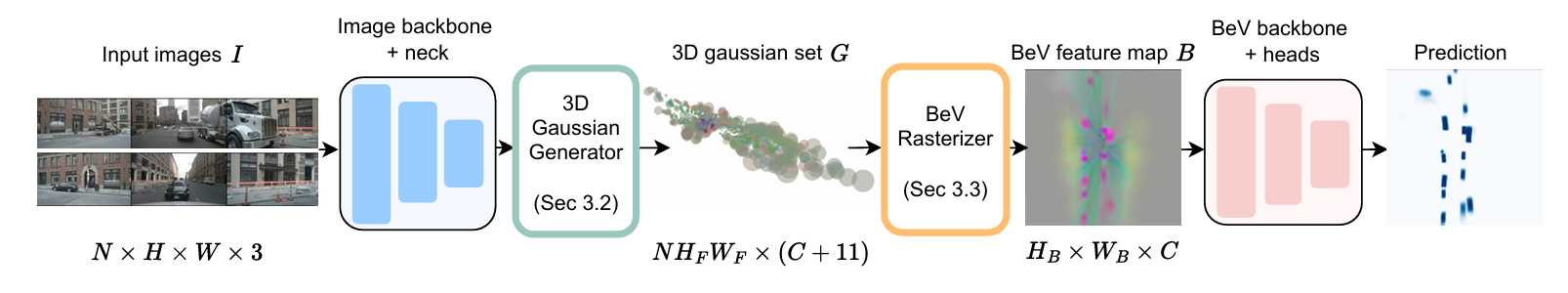
전체 파이프라인 개요
큰 그림은 의외로 단순하다. 네 덩어리로 끊어 읽으면 된다.
- Backbone으로 멀티카메라 이미지에서 feature map을 뽑는다.
- Gaussian Generator가 그 feature map의 픽셀마다 하나의 3D Gaussian을 예측한다 — 위치, 크기, 방향(quaternion), 불투명도, 그리고 $C$차원 feature embedding까지.
- 모든 카메라에서 나온 Gaussian들을 world frame에 모아, orthographic splatting으로 BEV 평면에 렌더링한다 → BEV feature map.
- 그 위에 BEV backbone + segmentation head를 얹어 최종 BEV semantic map을 낸다.
학습은 end-to-end다. BEV segmentation loss의 gradient가 differentiable rasterizer를 거쳐 Gaussian 파라미터 예측 head까지 그대로 흐른다. 아래에서 ②(Gaussian을 어떻게 예측하나)와 ③(어떻게 splat하나)를 수식으로 뜯어본다.
① Gaussian Generator — 픽셀 하나를 Gaussian 하나로
핵심은 여기다. feature map의 픽셀 $(u_{n,i}, v_{n,i})$ 하나하나가 3D Gaussian 하나가 된다($n$은 카메라 인덱스, $i$는 픽셀 인덱스). 한 Gaussian이 들고 가는 속성은 다섯 가지이고, 각각 전용 prediction head(Conv-BN-ReLU 두 블록짜리 가벼운 CNN)가 픽셀마다 뱉어낸다.
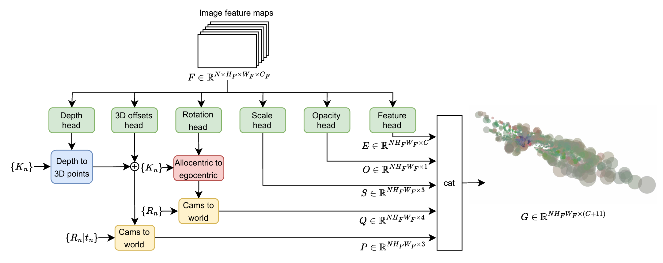
| 속성 | 기호 | 차원 | activation |
|---|---|---|---|
| Position | $P$ | 3 | (depth + offset으로 유도) |
| Scale | $S$ | 3 | absolute value |
| Rotation | $Q$ | 4 (quaternion) | L2 normalize |
| Opacity | $O$ | 1 | sigmoid |
| Embedding | $E$ | $C$ (=128) | — |
즉 generator의 출력은 픽셀당 $C+11$차원($3+3+4+1$ = 11)이고, 전체로는 $G \in \mathbb{R}^{N H_x W_x \times (C+11)}$ 텐서다. 이 중 가장 공들인 부분은 단연 position $P$다 — Gaussian이 3D 공간 어디에 놓이는지가 BEV 품질을 좌우하기 때문이다.
position은 두 단계로 만든다. 먼저 픽셀을 depth로 back-projection하고, 그 위에 학습된 3D offset을 더해 보정한다.
(1) depth로 back-projection. depth head는 픽셀마다 정규화된 disparity $d_{n,i} \in [0,1]$를 예측하고, 이를 metric depth $z_{n,i}$로 디코딩한다 (paper Eq. 1).
그리고 camera intrinsic $K_n$로 픽셀을 3D 카메라 좌표로 들어 올린다 (paper Eq. 2).
여기까지는 LSS의 lift와 본질이 같다 — 픽셀을 depth만큼 ray를 따라 밀어낸 것이다.
(2) 3D offset으로 보정. 그런데 depth 하나로 찍은 점은 ray 위에만 놓일 수 있어 자유도가 부족하다. 그래서 offset head가 픽셀마다 displacement $\Delta_{n,i} = (\Delta x, \Delta y, \Delta z)$를 예측해 점을 ray 바깥으로도 움직일 수 있게 한다 (paper Eq. 3).
마지막으로 extrinsic $[R_n \mid t_n]$으로 world frame에 옮기면 최종 position이다 (paper Eq. 4).
📐 잠깐 — depth만으로 충분하지 않은 이유. LSS류는 픽셀을 ray 위 한 점(또는 ray 위 분포)으로만 놓는다. 하지만 한 픽셀이 담는 물체의 표면은 ray에 딱 수직이지 않고 비스듬할 때가 많다. depth만 쓰면 Gaussian이 전부 ray 방향으로만 줄지어 서고, scale·rotation을 붙여도 “ray에 갇힌” 모양이 된다. 작은 $\Delta$ offset 하나를 더해 점을 ray 옆으로도 밀 수 있게 하면, Gaussian들이 실제 물체 표면을 따라 더 자연스럽게 깔린다. ablation에서 offset 제거 시 IoU가 47.1 → 46.9로 떨어지는데(작지만 일관됨), “ray에 갇히지 않게 하는” 이 자유도의 효과로 읽힌다.
나머지 속성도 짚어두자. rotation은 allocentric quaternion으로 예측한다 — 카메라가 물체를 보는 방향(viewing ray)에 따라 같은 물체도 이미지상 회전이 달라지는데, 이를 보정해 물체 자체의 방향만 학습하게 하는 트릭이다(monocular 3D detection에서 흔히 쓰는 그 allocentric/egocentric 구분과 같다). scale·opacity·embedding은 각 head가 곧장 regression한다. 특히 embedding $E$($C=128$)가 바로 나중에 색 대신 splat될 feature다.
② Splatting — Gaussian을 위에서 내려다보며 뭉갠다
이제 world frame에 수십만 개의 Gaussian이 떠 있다. 각 Gaussian은 위치 $\mathbf{p}^w$, 공분산($S, Q$로 결정), opacity $O$, feature $E$를 들고 있다. 이것을 BEV feature map으로 바꾸는 게 splatting이다.
원조 3DGS와의 결정적 차이는 시점이다. 3DGS는 카메라의 perspective 시점에서 splat해 사진을 만든다. GaussianBeV는 위에서 수직으로 내려다보는 orthographic 시점에서 splat한다 — BEV는 원근이 없는 평면 지도이므로 orthographic projection이 자연스럽다. 그리고 색(RGB) 대신 $C$차원 feature를 렌더링한다. 나머지 메커니즘(각 Gaussian을 평면에 투영해 2D 타원으로 만들고, opacity 가중으로 alpha-blending하는 미분 가능한 rasterization)은 Kerbl et al.(2023)의 그것을 그대로 차용한다.
결과는 $B \in \mathbb{R}^{H_B \times W_B \times C}$ 크기의 BEV feature map이다. 실험에서는 $200 \times 200$ 격자로, 100m × 100m 영역을 50cm 해상도로 덮는다. 이 feature map 위에 BEV backbone과 segmentation head를 얹어 최종 출력을 낸다.
🤔 (사견) 이 구조가 novel한 지점. LSS는 픽셀을 ray 위 점들로 흩뿌린 뒤 BEV 격자에 sum/pooling으로 모은다 — 어느 점이 어느 칸에 떨어지느냐는 hard한 양자화다. GaussianBeV는 그 대신 각 점을 면적과 방향을 가진 타원체로 만들어 부드럽게 격자에 번지게 한다. 같은 “splat”이라는 단어를 쓰지만, LSS의 splat이 점→격자 누적이라면 GaussianBeV의 splat은 타원체→평면 렌더링이다. 픽셀 하나가 BEV에서 한 칸이 아니라 제 모양대로 번지는 셈이라, 비스듬한 물체나 격자 경계에 걸린 물체가 덜 뭉개진다 — 앞서 말한 “격자 양자화 한계”를 정면으로 겨눈 설계다. 한 줄로 비유하면, Mip-NeRF가 NeRF의 point를 Gaussian으로 부풀려 aliasing을 눌렀듯이, GaussianBeV는 LSS의 point를 Gaussian으로 부풀려 격자 양자화를 누른다.
③ Loss — segmentation이 주, depth는 보조
학습 신호는 세 갈래로 들어간다.
(1) BEV semantic loss. 최종 BEV map에 거는 메인 loss로, 세 항의 가중합이다 (paper Eq. 7).
$\mathcal{L}_\text{bce}$가 segmentation 본체이고, $\mathcal{L}_\text{ctr}$(centerness)·$\mathcal{L}_\text{off}$(offset)는 보조 항이다.
(2) Early supervision. 영리한 한 수인데, 먼저 오해부터 풀자 — 이건 “BEV backbone에 loss를 건다”가 아니다. loss는 언제나 head의 출력(예측한 segmentation)에 걸린다. 핵심은 segmentation head가 두 개라는 점이다.
rasterizer
   │
   ├──→ [head_early] ──→ 예측A ──→ L_sem^early   ← raw BEV feature에 바로
   │
[BEV backbone]
   │
   └──→ [head_main]  ──→ 예측B ──→ L_sem         ← 정돈된 BEV feature에
두 갈래의 head — rasterizer 직후(raw BEV feature)에 붙는 early head와, BEV backbone을 거친 뒤의 main head. loss는 backbone이 아니라 각 head의 예측에 걸린다.
- main head : BEV backbone을 거친 뒤 정돈된 feature에서 segmentation을 예측 → 여기 걸리는 게 $\mathcal{L}_\text{sem}$.
- early head : BEV backbone을 거치기 전, rasterizer가 막 뱉은 raw BEV feature에 같은 형식의 head를 하나 더 붙여 segmentation을 예측 → 여기 걸리는 게 $\mathcal{L}_\text{sem}^\text{early}$.
즉 “BEV backbone에 loss를 준다”가 아니라, backbone 앞 지점에서도 한 번 segmentation을 예측하게 하고 그 예측에 loss를 거는 것이다. (그냥 간단하게 말해 auxiliary head 하나를 더 붙인 것) 최종 loss($\mathcal{L}_\text{sem}$)는 main head → BEV backbone → rasterizer → generator로 거꾸로 한참 흘러서야 generator에 닿는데, 경로가 길면 “Gaussian을 잘 예측하라”는 gradient가 backbone을 지나며 희석된다. early head는 backbone을 건너뛰고 바로 gradient를 꽂기 때문에, generator에 훨씬 직접적이다 — “raw BEV feature 만으로도 segmentation이 그럴듯해야 한다 = Gaussian이 그 자체로 옳게 예측돼 있어야 한다”를 강제하는 셈이다. (이 “head가 두 개”라는 구조 때문에, 뒤 ablation에서 early supervision이 BEV backbone이 있을 때만 효과를 내는 것도 자연스럽게 설명된다 — backbone이라는 긴 경로가 있어야 그걸 우회하는 지름길이 의미를 갖기 때문이다.)
(3) Depth loss. depth 예측을 LiDAR 등에서 얻은 GT depth $z^*$로 직접 지도한다 — log L1 형태다 (paper Eq. 8).
최종 loss는 셋의 합이다 (paper Eq. 9).
⚠️ ablation이 말해주는 미묘한 진실 — depth·early supervision은 “혼자서는” 안 듣는다. Table 4를 뜯어보면 흥미롭다. depth supervision만 단독으로 켜거나, early supervision만 단독으로 켜면 유의미한 이득이 없다. 그런데 BEV backbone과 함께, depth와 early supervision을 둘 다 켜면 그제야 47.0 → 47.5로 오른다. 즉 이 보조 신호들은 독립적인 마법이 아니라, 메인 경로가 갖춰진 위에서 같이 작동할 때만 효과가 난다. (rotation head 제거 −0.4, offset 제거 −0.2도 비슷한 결로, 개별 기여는 작고 합쳐서 효과를 낸다. 즉 이 논문의 성능은 한 방의 트릭이 아니라 “Gaussian 표현 자체”에서 온다는 방증이기도 하다.)
nuScenes Benchmark & Results
평가는 nuScenes vehicle BEV semantic segmentation, metric은 IoU다. 모두 single-frame(temporal 미사용) 세팅이며, visibility > 40% 필터 기준이다.
저해상도 (224×448):
| Method | Vehicle IoU |
|---|---|
| BEVFormer | 42.0 |
| Simple-BEV | 43.0 |
| PointBeV | 44.0 |
| GaussianBeV | 47.5 |
고해상도 (448×800):
| Method | Vehicle IoU |
|---|---|
| PointBeV | 47.6 |
| GaussianBeV | 50.3 |
읽는 법은 간단하다.
- 같은 조건에서 일관되게 앞선다. 224×448에서 PointBeV 대비 +3.5 (44.0 → 47.5), 448×800에서 +2.7 (47.6 → 50.3). 당시 SOTA를 두 해상도 모두에서 갈아치웠다.
- 이득의 출처가 명확하다. ablation상 보조 loss들의 기여(±0.5 안팎)를 다 합쳐도 격차의 일부일 뿐이다. 나머지는 “BEV를 격자가 아니라 oriented Gaussian의 집합으로 표현한다”는 본체에서 온다.
Conclusion — 픽셀을 격자가 아니라 Gaussian으로
정리하면, GaussianBeV의 기여는 이렇다.
scene별 최적화가 필요했던 3D Gaussian Splatting을, 네트워크가 단 한 번의 forward로 Gaussian들을 통째로 예측하게 만들어 online image→BEV 변환에 끼워 넣었다. 픽셀 하나를 격자 칸이 아니라 위치·방향·크기를 가진 3D 타원체 하나로 보고, 그것들을 orthographic하게 splat해 BEV feature를 렌더링한다.
이 시리즈의 출발점으로서 GaussianBeV가 던지는 메시지는 분명하다 — BEV feature는 격자 양자화의 산물일 필요가 없다. 연속 공간에 자유롭게 놓인 Gaussian들의 렌더링으로 만들 수 있고, 그게 더 또렷한 형상을 담는다.
다만 한 걸음 물러서서 보면, 이 출발점에는 다음 논문들이 파고들 틈도 함께 보인다. 첫째, 각 Gaussian의 위치가 결국 depth 예측에 크게 의존한다 — depth가 흔들리면 Gaussian이 엉뚱한 곳에 놓이고 BEV도 같이 무너진다(다음 글 GaussianLSS가 정확히 이 depth의 불확실성을 정면으로 다룬다). 둘째, 여기서 각 Gaussian이 드는 feature는 BEV task loss로만 간접 지도될 뿐, 그 Gaussian이 실제 3D 기하를 옳게 잡았는지 직접 검증받지 않는다 — RGB로 렌더링해 맞춰보거나(reconstruction), appearance를 함께 들게 하는 후속 흐름이 여기서 갈라져 나온다.
그럼에도 “픽셀 = oriented 3D Gaussian”이라는 단순하고 강한 한 줄은, 이후 BEV-Gaussian 연구들이 공유하는 공통 어휘가 되었다. 시리즈의 첫 단추로 더없이 적절한 논문이다.
읽어주셔서 감사합니다. 혹시 제가 잘못 이해한 부분이 있다면 언제든 알려주세요 :)
Figure sources are linked inline :)
+++ First post in the Gaussian Splatting for BEV Perception section. This series follows the answers that recent 3D Gaussian Splatting has offered to an old question — “how should we build the BEV feature?” The starting point is GaussianBeV: the first attempt to slot 3DGS, originally a tool for scene reconstruction, into image→BEV transformation in a single forward pass, with no per-scene optimization. The idea: treat each image pixel as a tiny oriented ellipsoid (a Gaussian) floating in 3D, and splat them as seen from above — that gives you a BEV feature. 🚀
GaussianBeV: 3D Gaussian Representation meets Perception Models for BeV Segmentation
Authors : Florian Chabot, Nicolas Granger, Guillaume Lapouge (CEA-List, Université Paris-Saclay · CEA–Valeo joint lab)
Venue : WACV 2025
Paper Link : https://arxiv.org/abs/2407.14108
Code : not released (no official implementation)
Introduction & Motivation
image → BEV: who has done this transform, and how?
Nearly every autonomous-driving perception pipeline hits the same problem at one point — how to move the perspective images from several cameras into a single top-down BEV (Bird’s-eye View) plane. Whether the downstream task is detection, segmentation, or topology reasoning, its fate largely rides on how good this BEV feature is.
Two families had crystallized for solving that transform.
- Lift-Splat-Shoot (LSS) family — “lift the pixels.” Predict a depth distribution per pixel, scatter the feature along the camera ray according to it (lift), then drop them into the BEV grid and pool (splat). Depth is explicit, so geometry is sharp, but treating depth as a distribution over discrete bins makes the representation coarse.
- BEVFormer / Simple-BEV family — “look back from BEV.” Fix each cell (query) of the BEV grid, project it to where it should look in the image, and gather features (attention or bilinear sampling). No explicit depth, so it’s stable, but the 3D geometry is implicit and object shape/orientation gets blurred.
Both families share a weakness — they ultimately quantize the scene into a fixed grid (voxel / BEV cell). A grid is bound by its resolution, and the smaller or more slanted the object (pedestrians, the corner of a car), the more it smears at cell boundaries.
So they bring in 3D Gaussian Splatting
GaussianBeV’s idea starts here. As it happens, 3D Gaussian Splatting (3DGS) had risen on the graphics side — represent a scene with hundreds of thousands of tiny 3D ellipsoids (Gaussians), each carrying position, shape, orientation, opacity, and color, and splat them along the camera’s viewing direction to render a photo. Because these are points floating freely in continuous space rather than a grid, the grid-quantization limit disappears.
But vanilla 3DGS has one decisive constraint that blocks direct use in BEV perception — it requires thousands of optimization steps per individual scene for the Gaussians to settle. In driving, every frame is an unseen scene; you can’t run an optimization per frame.
GaussianBeV’s one-line contribution lands exactly here.
Drop the per-scene optimization. Instead, let a network look at the images and predict, in a single forward pass, the whole set of “Gaussians that make up this scene.” Then splat those Gaussians from an orthographic top-down view (not the camera view), rendering features instead of colors — and that is the BEV feature map.
In the authors’ words, this is the first approach to integrate 3D Gaussian modeling and 3D scene rendering online, within a single-stage model, without per-scene optimization — though, to be precise, “first” means first in BEV perception, not that the idea of “GS without per-scene optimization” itself is new (see the box below). Where LSS “lifts” pixels onto rays, GaussianBeV turns each pixel into a single oriented ellipsoid placed in 3D space. That is the whole — and the core — of this paper.
🤔 A quick aside — isn’t this just feed-forward GS? Yes. The skeleton — “drop per-scene optimization, and let a network regress a Gaussian per pixel in one forward pass” — is identical to feed-forward GS (Splatter Image, PixelSplat, MVSplat, etc.). GaussianBeV doesn’t invent a new GS paradigm; it’s the first to bring existing feed-forward GS into BEV perception. So the “predict a pixel-aligned Gaussian per pixel” part is exactly the same. What diverges is what, how, and against what it renders.
(My take) To be fair, the paper doesn’t entirely bury feed-forward GS — PixelSplat and Splatter Image are in the references, and its “first” claim is precisely worded as “the first time a not-scene-specific GS representation is proposed and integrated into a BeV perception model”, scoped to BEV (it does not claim a first in GS at large). Still: GaussianBeV v1 appeared in July 2024, by which point PixelSplat (Dec 2023), Splatter Image (Nov 2023), and MVSplat (Mar 2024) were an established line, already at CVPR/ECCV. Yet the Related Work’s “Gaussian splatting” subsection discusses only per-scene-optimized 3DGS and barely engages this feed-forward lineage. Citing them but never spelling out in the body “how our method is the same as, and differs from, that line” leaves a reader prone to over-reading the contribution — if I were a reviewer, I’d have pushed back a little here.)
- Render target: vanilla feed-forward GS renders RGB (color/SH) to make novel-view images. GaussianBeV drops RGB and renders a $C$-dimensional task feature.
- Render viewpoint: the former is perspective (novel camera view), the latter orthographic top-down (BEV).
- Supervision: the former uses photometric reconstruction (match the rendered image to GT photos), the latter a BEV segmentation loss (the task drives learning). That is, GaussianBeV has no photometric loss.
That last line matters. A vanilla feed-forward GS’s Gaussians are verified directly by “did you reconstruct RGB correctly,” but GaussianBeV’s Gaussians never get that check — whether the geometry is right is confirmed only indirectly, through the BEV task loss (plus the auxiliary depth loss). This “absence of direct geometric verification” is the starting point for later papers to bring RGB rendering back (the second “crack” in this post’s conclusion).
Method
Pipeline overview
The big picture is surprisingly simple. Read it in four chunks.
- A backbone extracts feature maps from the multi-camera images.
- A Gaussian Generator predicts one 3D Gaussian per pixel of that feature map — position, scale, orientation (quaternion), opacity, and a $C$-dimensional feature embedding.
- The Gaussians from all cameras are gathered in the world frame and rendered onto the BEV plane via orthographic splatting → a BEV feature map.
- A BEV backbone + segmentation head on top produces the final BEV semantic map.
Training is end-to-end: the gradient of the BEV segmentation loss flows through the differentiable rasterizer all the way back to the Gaussian-parameter heads. Below we dissect ② (how Gaussians are predicted) and ③ (how they are splatted) with equations.
① Gaussian Generator — one pixel into one Gaussian
This is the heart of it. Each pixel $(u_{n,i}, v_{n,i})$ of the feature map becomes one 3D Gaussian ($n$ is the camera index, $i$ the pixel index). A Gaussian carries five attributes, each emitted per pixel by a dedicated prediction head (a light CNN of two Conv-BN-ReLU blocks).
| Attribute | Symbol | Dim | activation |
|---|---|---|---|
| Position | $P$ | 3 | (derived from depth + offset) |
| Scale | $S$ | 3 | absolute value |
| Rotation | $Q$ | 4 (quaternion) | L2 normalize |
| Opacity | $O$ | 1 | sigmoid |
| Embedding | $E$ | $C$ (=128) | — |
So the generator outputs $C+11$ dims per pixel ($3+3+4+1$ = 11), giving a tensor $G \in \mathbb{R}^{N H_x W_x \times (C+11)}$. The most carefully designed piece is by far the position $P$ — where a Gaussian sits in 3D determines the BEV quality.
Position is built in two stages. First back-project the pixel via depth, then refine it with a learned 3D offset.
(1) Back-project via depth. The depth head predicts a normalized disparity $d_{n,i} \in [0,1]$ per pixel and decodes it to metric depth $z_{n,i}$ (paper Eq. 1).
Then the camera intrinsic $K_n$ lifts the pixel to a 3D camera-frame point (paper Eq. 2).
This is essentially LSS’s lift — pushing the pixel along the ray by its depth.
(2) Refine with a 3D offset. But a point placed by depth alone can only lie on the ray, which is too few degrees of freedom. So the offset head predicts a displacement $\Delta_{n,i} = (\Delta x, \Delta y, \Delta z)$ per pixel, letting the point move off the ray too (paper Eq. 3).
Finally the extrinsic $[R_n \mid t_n]$ moves it to the world frame — the final position (paper Eq. 4).
📐 A quick aside — why depth alone isn’t enough. LSS-style methods place a pixel only on the ray (a point, or a distribution along it). But the object surface a pixel captures is often slanted, not perpendicular to the ray. With depth alone, every Gaussian lines up along the ray direction, and even with scale/rotation attached the shape stays “trapped on the ray.” Adding a small $\Delta$ offset that nudges the point off to the side of the ray lets the Gaussians drape along the actual object surface more naturally. In the ablation, removing the offset drops IoU 47.1 → 46.9 (small but consistent), readable as the effect of this “un-trap from the ray” degree of freedom.
A note on the rest. Rotation is predicted as an allocentric quaternion — the same object appears rotated differently in the image depending on the viewing ray, and predicting allocentrically factors that out so the head learns the object’s own orientation (the same allocentric/egocentric distinction common in monocular 3D detection). Scale, opacity, embedding are regressed directly by their heads. In particular, the embedding $E$ ($C=128$) is exactly the feature that will later be splatted in place of color.
② Splatting — squash the Gaussians as seen from above
Now hundreds of thousands of Gaussians float in the world frame. Each carries a position $\mathbf{p}^w$, a covariance (from $S, Q$), opacity $O$, and feature $E$. Turning these into a BEV feature map is the splatting.
The decisive difference from vanilla 3DGS is the viewpoint. 3DGS splats from the camera’s perspective view to make a photo. GaussianBeV splats from an orthographic top-down view — BEV is a perspective-free planar map, so orthographic projection is the natural fit. And it renders $C$-dimensional features instead of color (RGB). The rest of the machinery (project each Gaussian to the plane as a 2D ellipse, alpha-blend with opacity weighting, all differentiable) is borrowed straight from Kerbl et al. (2023).
The result is a BEV feature map $B \in \mathbb{R}^{H_B \times W_B \times C}$. In experiments it’s a $200 \times 200$ grid covering a 100m × 100m area at 50cm resolution. A BEV backbone and segmentation head on top produce the final output.
🤔 (My take) Where this design is novel. LSS scatters a pixel into points along the ray, then aggregates them into the BEV grid by sum/pooling — which point lands in which cell is a hard quantization. GaussianBeV instead makes each point an ellipsoid with area and orientation that bleeds softly into the grid. Same word “splat,” but LSS’s splat is a point→grid accumulation, while GaussianBeV’s is an ellipsoid→plane rendering. A single pixel spreads in BEV not as one cell but according to its own shape, so slanted objects or objects straddling cell boundaries smear less — a design aimed squarely at the “grid-quantization limit” noted earlier. In one line: just as Mip-NeRF inflates NeRF’s point into a Gaussian to suppress aliasing, GaussianBeV inflates LSS’s point into a Gaussian to suppress grid quantization.
③ Loss — segmentation primary, depth auxiliary
The training signal enters along three paths.
(1) BEV semantic loss. The main loss on the final BEV map, a weighted sum of three terms (paper Eq. 7).
$\mathcal{L}_\text{bce}$ is the segmentation core; $\mathcal{L}_\text{ctr}$ (centerness) and $\mathcal{L}_\text{off}$ (offset) are auxiliary.
(2) Early supervision. A clever move — but first, a misconception to clear up: this is not “putting a loss on the BEV backbone.” A loss is always applied to a head’s output (the predicted segmentation). The key is that there are two segmentation heads.
rasterizer
   │
   ├──→ [head_early] ──→ pred A ──→ L_sem^early   ← on the raw BEV feature
   │
[BEV backbone]
   │
   └──→ [head_main]  ──→ pred B ──→ L_sem         ← on the polished BEV feature
Two heads — an early head on the raw BEV feature right after the rasterizer, and the main head after the BEV backbone. The loss is applied to each head’s prediction, not to the backbone.
- main head: predicts segmentation from the polished feature after the BEV backbone → this is where $\mathcal{L}_\text{sem}$ is applied.
- early head: before the BEV backbone, a second head of the same form is attached to the raw BEV feature the rasterizer just emitted, predicting segmentation → this is where $\mathcal{L}_\text{sem}^\text{early}$ is applied.
So it’s not “a loss on the BEV backbone” but making a segmentation prediction at the pre-backbone point too, and putting a loss on that prediction. (Put simply, it’s just one extra auxiliary head.) This is the common technique of deep supervision (auxiliary heads). The final loss ($\mathcal{L}_\text{sem}$) only reaches the generator after flowing all the way back through main head → BEV backbone → rasterizer → generator; the longer the path, the more the “predict good Gaussians” gradient is diluted passing through the backbone. The early head skips the backbone and injects gradient straight in, so that demand lands on the generator far more directly — it forces “segmentation must look right from the raw BEV feature alone = the Gaussians must already be predicted correctly on their own.” (This “two heads” structure also naturally explains why, in the ablation below, early supervision helps only when the BEV backbone is present — a shortcut is only meaningful when there’s a long path to short-cut around.)
(3) Depth loss. Supervise the depth prediction directly with GT depth $z^*$ (e.g. from LiDAR) — a log-L1 form (paper Eq. 8).
The total loss is the sum of the three (paper Eq. 9).
⚠️ A subtle truth from the ablation — depth and early supervision don’t help “on their own.” Table 4 is telling. Turning on depth supervision alone, or early supervision alone, yields no meaningful gain. But with the BEV backbone, turning on both depth and early supervision finally lifts 47.0 → 47.5. So these auxiliary signals aren’t independent magic; they work only when fired together on top of an established main path. (Removing the rotation head −0.4 and the offset −0.2 are similar in spirit — each individual contribution is small, and they add up.) This is also evidence that the paper’s performance comes not from one trick but from “the Gaussian representation itself.”
nuScenes Benchmark & Results
Evaluation is nuScenes vehicle BEV semantic segmentation, metric IoU. All numbers are single-frame (no temporal), under the visibility > 40% filter.
Low resolution (224×448):
| Method | Vehicle IoU |
|---|---|
| BEVFormer | 42.0 |
| Simple-BEV | 43.0 |
| PointBeV | 44.0 |
| GaussianBeV | 47.5 |
High resolution (448×800):
| Method | Vehicle IoU |
|---|---|
| PointBeV | 47.6 |
| GaussianBeV | 50.3 |
How to read it:
- It leads consistently under matched conditions. +3.5 over PointBeV at 224×448 (44.0 → 47.5), +2.7 at 448×800 (47.6 → 50.3). It set the SOTA at both resolutions at the time.
- The source of the gain is clear. Summing all the auxiliary-loss contributions (around ±0.5) accounts for only part of the gap. The rest comes from the core idea — representing BEV as a set of oriented Gaussians rather than a grid.
⚠️ Caution when comparing. This table is all single-frame, visibility>40%. Don’t compare it directly to numbers from papers that use temporal or a different visibility filter — BEV segmentation IoU swings a lot with these two settings. (Same spirit as the earlier series’ warning against cross-version comparison on the OpenLane-V2 metric.)
Conclusion — pixels as Gaussians, not grid cells
To sum up, GaussianBeV’s contribution is this.
It takes 3D Gaussian Splatting — which used to require per-scene optimization — and makes a network predict the whole set of Gaussians in a single forward pass, slotting it into online image→BEV transformation. A pixel is seen not as a grid cell but as one 3D ellipsoid with position, orientation, and scale, and these are splatted orthographically to render the BEV feature.
As the series’ starting point, GaussianBeV’s message is clear — a BEV feature need not be a product of grid quantization. It can be made by rendering Gaussians placed freely in continuous space, and that captures sharper shapes.
Step back, though, and this starting point also reveals the cracks the next papers will dig into. First, each Gaussian’s position ultimately depends heavily on depth prediction — if depth wobbles, the Gaussian lands in the wrong place and the BEV collapses with it (the next post, GaussianLSS, tackles exactly this uncertainty of depth head-on). Second, the feature each Gaussian carries is only indirectly supervised by the BEV task loss; whether that Gaussian actually got the 3D geometry right is never directly verified — and the follow-up lines that render with RGB to check (reconstruction), or make Gaussians also carry appearance, branch off here.
Even so, the simple, strong one-liner “pixel = oriented 3D Gaussian” became the shared vocabulary of the BEV-Gaussian works that followed. As the first button of the series, it’s a fitting paper indeed.
Thanks for reading. If I’ve misunderstood anything, please let me know :)
comments