GaussianLSS — Toward Real-world BEV Perception: Depth Uncertainty Estimation via Gaussian Splatting
Paper review · depth를 한 점이 아니라 분포로 보고, 그 분산을 3D Gaussian의 covariance로 흘려보낸다.
각 figure의 출처는 하이퍼링크로 달아두었습니다 :)
+++ Gaussian Splatting for BEV Perception 섹션의 두 번째 글이다. 앞 글(GaussianBeV)에서 두 가지 문제점을 짚어뒀다 — (1) Gaussian의 위치가 depth 예측에 크게 의존한다, (2) Gaussian이 geometry를 옳게 잡았는지 직접 검증받지 않는다. GaussianLSS는 그중 첫 번째를 정면으로 받는다. 답하는 방식이 흥미로운데, depth를 더 정확히 맞히려 들지 않는다. 대신 “depth는 어차피 틀린다, 그러니 틀린 정도(uncertainty)를 표현에 그대로 녹이자”로 방향을 튼다. 그리고 그 uncertainty를 3D Gaussian의 covariance로 흘려보낸다.
GaussianLSS — Toward Real-world BEV Perception: Depth Uncertainty Estimation via Gaussian Splatting
Authors : Shu-Wei Lu, Yi-Hsuan Tsai, Yi-Ting Chen (National Yang Ming Chiao Tung University · Atmanity Inc.)
Venue : CVPR 2025
Paper Link : https://arxiv.org/abs/2504.01957
Code : https://github.com/HCIS-Lab/GaussianLSS (공식, MIT)
Introduction & Motivation
LSS의 depth는 왜 불안한가
출발점은 다시 LSS다. 앞 글에서 봤듯 LSS는 픽셀마다 depth 분포를 예측해 feature를 ray 위로 흩뿌린다. 여기서 그 “depth 분포”가 어떻게 생겼는지를 한 겹 더 들여다보면 문제가 보인다.
LSS는 depth를 연속값으로 regression하지 않는다. depth 축을 $B$개의 bin으로 잘라놓고(예: 1m, 2m, …, 60m), 각 bin에 대한 확률을 softmax로 뽑는 categorical 분류로 푼다. feature는 이 확률로 가중되어 각 bin 위치에 흩뿌려진다.
문제는 이 categorical 표현이 불안정하다는 데 있다. 실제 depth가 두 bin 경계 근처에 있으면, 거의 같은 거리인데도 softmax 확률이 인접 bin 사이에서 크게 출렁인다. 같은 물체의 비슷한 깊이가 frame마다, 픽셀마다 다른 bin으로 튀고, 그 결과 BEV에 떨어지는 feature도 들쭉날쭉해진다. depth를 “어느 칸이냐”로 강제 양자화한 대가다. (앞 글에서 GaussianBeV가 격자 양자화를 지적했다면, 여기선 그 양자화가 depth 축에서 일어나는 셈이다.)
게다가 이런 unprojection 계열은 결국 depth를 잘 맞혀야 BEV가 산다. depth가 틀리면 feature가 엉뚱한 칸에 떨어진다. 그래서 보통 LiDAR depth로 보조 supervision까지 걸어가며 depth 정확도에 매달리는데 — 현실의 depth는 본질적으로 ambiguous하다. 한 픽셀이 담는 게 가까운 물체의 가장자리인지 먼 배경인지, 단안 카메라로는 애초에 단정할 수 없는 경우가 많다.
“정확히 맞히기” 대신 “틀린 정도를 표현하기”
GaussianLSS의 방향 전환이 여기서 나온다. depth ambiguity를 없애야 할 오차로 보지 않는다. 오히려 표현해야 할 정보로 본다.
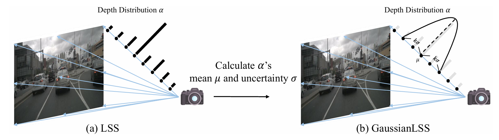
depth를 한 점($\mu$)이 아니라 분포로 보고, 그 분포의 분산($\sigma^2$)까지 함께 들고 간다. 분산이 크다는 건 “이 픽셀의 depth는 불확실하다”는 뜻이고, 그 불확실성을 3D 공간의 퍼짐(spatial extent)으로 번역해 3D Gaussian의 covariance에 담는다.
직관은 이렇다. depth가 확실한 픽셀(예: 가까운 차의 표면)은 3D에서 한 점에 가깝게 모인다 → 작은 covariance. depth가 불확실한 픽셀(예: 멀거나 경계가 모호한 곳)은 ray를 따라 넓게 퍼진 형태가 된다 → 길쭉한 covariance. 즉 covariance의 모양이 곧 그 픽셀이 표현하는 물체의 불확실한 퍼짐을 나타낸다. 저자들은 이 covariance가 supervision 없이도 object extent를 implicit하게 잡아낸다고 말한다.
이게 왜 유용하냐? — depth를 “정확히 한 점으로” 맞혀야 하는 부담을 덜어준다. $[\mu - k\sigma,\ \mu + k\sigma]$라는 soft한 범위로 풀어두면, depth가 조금 어긋나도 그 범위가 실제 물체를 덮을 가능성이 높다. “depth 정확도에 대한 의존을 낮춘다”가 이 논문이 abstract에서 내세우는 바로 그 문장이다.
GaussianBeV와 무엇이 다른가
같은 “Gaussian으로 BEV” 계열이지만, 두 논문은 Gaussian을 만드는 출발점이 다르다.
- GaussianBeV : 픽셀마다 Gaussian의 속성(위치·scale·rotation·opacity·feature)을 head로 직접 regression한다. 위치는 depth + 3D offset으로 찍는다. Gaussian의 covariance(scale·rotation)도 네트워크가 직접 예측한다.
- GaussianLSS : Gaussian의 mean과 covariance를 직접 예측하지 않는다. depth 분포에서 통계적으로 유도한다 — 분포의 평균이 mean, 분포의 분산이 covariance다. 즉 covariance가 “학습된 모양”이 아니라 “depth 불확실성의 기하적 번역”이다.
방향이 정반대다. GaussianBeV가 “Gaussian을 더 자유롭게 예측하자”였다면, GaussianLSS는 “Gaussian을 depth 분포에서 유도하되, 그 분포의 불확실성을 버리지 말고 covariance로 살리자”다. 그래서 이 논문은 스스로를 GaussianBeV류가 아니라 LSS(unprojection) 계열의 재해석으로 위치시킨다 — 제목에 LSS가 들어간 이유다.
Method
전체 파이프라인 개요
순서대로 끊으면 이렇다.
- 6개 카메라 이미지를 backbone(EfficientNet-B4)으로 인코딩한다.
- 픽셀마다 세 가지를 뽑는다 — splat할 feature $F_i \in \mathbb{R}^C$, opacity $\alpha_i$, 그리고 depth 분포 $P_i$.
- depth 분포를 3D uncertainty 변환에 태워, 픽셀마다 3D Gaussian(mean $\mu_{3d}$ + covariance $\Sigma$)을 만든다.
- 이 Gaussian들을 uncertainty-weighted splatting으로 BEV 평면에 렌더링한다 (multi-scale).
- BEV feature 위에 task head(segmentation / detection)를 얹는다.
핵심은 ③의 변환과 ④의 splatting이다. 아래에서 수식으로 본다.
① depth 분포 → 3D Gaussian — 분산을 covariance로
픽셀 $p$의 depth 분포 $P_i(p)$는 $B$개 bin 위의 확률이다($d_i$는 $i$번째 bin의 depth). 여기서 두 통계량을 뽑는다 (paper Eq. 1–2).
$\mu$는 soft depth mean(기댓값), $\sigma^2$는 depth 분포의 분산이다. argmax로 한 bin을 고르는 게 아니라 분포 전체를 평균낸다는 점이 LSS의 categorical pick과 다른 첫 번째 지점이다 — 이미 여기서 bin 경계의 출렁임이 누그러진다.
그다음이 이 논문의 알맹이다. depth 통계를 3D 공간의 Gaussian으로 올린다. 각 bin의 depth $d_i$를 카메라 intrinsic $I$·extrinsic $E$로 unproject하면 3D 점 $p_i^{3d}$가 나오고, 그 점들의 분포로 3D mean과 covariance를 만든다 (paper Eq. 3–4).
코드(GaussianLSS/model/GaussianLSS.py의 pred_depth())도 정확히 이 두 줄이다 — depth를 softmax해 확률을 만들고, 3D 좌표를 그 확률로 가중평균하면 mean, 평균에서의 편차(delta_3d)의 외적을 가중합하면 covariance다.
# GaussianLSS/model/GaussianLSS.py — pred_depth()
depth_prob = depth.softmax(1)                                   # P_i(p)
pred_coords_3d = (depth_prob.unsqueeze(-1) * coords_3d).sum(1)   # μ_3d = Σ P_i · p_i^3d

delta_3d = pred_coords_3d.unsqueeze(1) - coords_3d
cov = (depth_prob[...,None,None] * (delta_3d.unsqueeze(-1) @ delta_3d.unsqueeze(-2))).sum(1)  # Σ
scale = (self.error_tolerance ** 2) / 9
cov = cov * scale                                               # k로 covariance 스케일
마지막 두 줄을 눈여겨보자. covariance에 $\text{(error\_tolerance)}^2/9$를 곱한다. 앞서 말한 error tolerance 계수 $k$가 여기서 covariance의 크기로 들어간다 — $/9$는 $3\sigma$ 규약($(k/3)^2$)에서 온 것으로, “$k\sigma$ 범위를 covariance로 환산”하는 장치다. 즉 $[\mu-k\sigma, \mu+k\sigma]$라는 soft 범위가 추상적 비유가 아니라 이 한 줄의 스케일링으로 실제 구현돼 있다.
여기서 $\Sigma$가 바로 depth 불확실성의 3D 번역이다. depth 분포가 한 bin에 뾰족하게 몰리면 $p_i^{3d}$들이 한 점에 모여 $\Sigma$가 작아지고, 분포가 넓게 퍼지면 $p_i^{3d}$들이 ray를 따라 늘어서 $\Sigma$가 그 방향으로 길쭉해진다. 즉 covariance의 주축이 ray 방향과 정렬되며, 그 길이가 depth 불확실성의 크기다.
📐 잠깐 — covariance가 ray를 따라 길쭉해지는 게 핵심이다. depth가 불확실한 픽셀에서 진짜 모르는 건 “ray 위 어디냐”이지, ray와 수직인 방향(이미지 평면상 위치)이 아니다. 이미지상 위치는 픽셀 좌표로 이미 정해져 있으니까. 그래서 불확실성은 자연히 ray 방향으로만 퍼지고, $\Sigma$도 그 방향으로 늘어난 타원체가 된다. 이게 “object extent를 implicit하게 잡는다”는 주장의 실체다 — 멀리 있어 depth가 모호한 물체일수록 Gaussian이 깊이 방향으로 길게 늘어나, 그 물체가 차지할 법한 범위를 자연스럽게 덮는다. (직접 extent를 regression하는 변형은 ablation에서 1.3%p 더 낮았다. 분포에서 유도하는 쪽이 낫다는 것.)
이 Gaussian이 드는 건 결국 geometry(mean·covariance) + opacity + feature다. RGB도, photometric loss도 없다. feature는 segmentation loss로 discriminative하게 학습될 뿐, 그 Gaussian이 실제 3D를 옳게 잡았는지는 직접 검증되지 않는다. 이 점은 뒤 Conclusion에서 다시 짚는다.
② Splatting — uncertainty로 가중해 BEV에 뭉갠다
각 픽셀이 3D Gaussian $G_i(x) = \alpha_i \exp\!\big(-\tfrac{1}{2}(x-\mu_i)^\top \Sigma_i^{-1}(x-\mu_i)\big)$ 하나를 만들었다. 이제 이걸 BEV 평면에 올린다.
렌더링은 색 대신 feature를 splat하는 것으로, 원조 3DGS의 color compositing(paper Eq. 4)에서 색 $c_i$를 feature $F_i$로 갈아끼운 형태다 (paper Eq. 5).
📌 표준 3DGS의 alpha blending과 미묘하게 다르다. 원조 3DGS는 depth로 정렬한 뒤 앞에서부터 합성하는 front-to-back alpha compositing인데, 해당 수식엔 transmittance 항 $T_i = \prod_{j \lt i}(1-\alpha_j)$가 들어간다 — “앞에 놓인 Gaussian들을 통과하고 남은 빛의 비율”로, 앞쪽이 불투명할수록 뒤쪽 기여가 줄어드는 occlusion을 표현한다. 그런데 위 Eq. 5엔 이 $T_i$가 없다 — 그냥 $\alpha_i$로 가중한 weighted sum이다. BEV는 top-down orthographic이라 “앞 Gaussian이 뒤를 가린다”는 occlusion ordering이 의미가 없기 때문이다. 위에서 수직으로 내려다보면 깊이 방향 앞뒤 가림을 따질 게 없으니, 순서에 의존하는 transmittance를 떼고 순서 무관한 가중합으로 단순화한 것이다. (때문에 3D-GS에서 제일 병목인 Gaussian을 depth로 sorting하는 과정도 필요없다.)
여기서 $\Sigma_i$가 가중에 직접 들어간다는 게 포인트다. covariance가 길쭉한(불확실한) Gaussian은 넓은 영역에 옅게 깔리고, 뾰족한(확실한) Gaussian은 좁은 영역에 진하게 박힌다. 불확실성이 splat의 모양과 세기를 직접 정한다. 메커니즘 자체는 GaussianBeV의 splat과 같고 — 다른 건 그 $\Sigma_i$를 어디서 가져오느냐다. GaussianBeV는 head로 직접 예측했지만, GaussianLSS는 ①에서 본 대로 depth 분포에서 유도한다. BEV로 내릴 때 covariance는 z축을 무시하고 2D로 투영된다($\Sigma' = S_\text{BEV}\,\Sigma_{xy}\,S_\text{BEV}^\top$).
splatting은 multi-scale로 한다(50×50, 100×100, 200×200). 단일 해상도로는 Gaussian 기반 표현이 projection 계열보다 물체 형상을 약간 뭉개는 경향이 있어서, 여러 해상도에서 렌더해 이를 보완한다. 최종 BEV는 200×200 격자로 [−50m, 50m] 범위를 덮는다.
🤔 (사견) opacity는 사실상 pruning 스위치다. 저자들이 흘리듯 적은 관찰이 흥미롭다 — 학습이 수렴하면 Gaussian의 80%가 opacity $\lt 0.01$로 떨어진다(§4.6, Fig. 7). 명시적 sparsity 항으로 누른 것도 아닌데 대부분의 픽셀-Gaussian이 “거의 안 보이는” 상태가 되고, 소수($\sim$20%)만 실제로 BEV에 기여한다. 그리고 이건 단순 관찰에 그치지 않는다 — 코드를 보면 렌더링 직전에 opacity가 임계(0.05) 미만인 Gaussian을 실제로 잘라내고(mask) rasterizer에 넘긴다.
# GaussianLSS/model/GaussianLSS.py — GaussianRenderer.forward()
mask = (opacities > self.threshold)   # threshold=0.05, 임계 미만은 버림
...
rendered_bev, _ = self.rasterizer(
    means3D = means3D[i][mask[i]],     # 살아남은 Gaussian만 렌더
    colors_precomp = features[i][mask[i]],
    opacities = opacities[i][mask[i]],
    cov3D_precomp = cov3D[i][mask[i]],
)
즉 “픽셀당 하나씩 Gaussian을 찍는다”는 설계가 결과적으로 80%가 죽는 과잉 표현이고, 그 죽은 Gaussian을 opacity 마스킹으로 실제로 걷어낸다. (어차피 대부분 버릴 거면 애초에 덜 찍는 구조가 더 깔끔하지 않았을까 — 다만 어느 픽셀이 살아남을지 미리 알 수 없으니 일단 다 찍고 학습이 알아서 죽이게 둔 뒤 임계로 거르는 게 현실적이긴 하다. 효율 수치의 일부는 여기서 온다.)
③ Loss — segmentation이 끌고, depth는 implicit하게
loss 구성은 단출하다 (paper 기준).
$\mathcal{L}_\text{focal}$이 segmentation 본체이고, $\mathcal{L}_\text{L1}\!\cdot\!\mathcal{L}_\text{L2}$는 centerness·offset 류의 보조 항이다.
주목할 건 명시적 depth supervision이 없다는 점이다. LSS류가 흔히 LiDAR depth로 depth head를 직접 지도하는 것과 달리, GaussianLSS는 depth 분포 $P_i$를 오직 segmentation loss를 통해 implicit하게 학습한다. depth를 직접 맞히라고 강제하지 않는 게 이 논문의 일관된 태도다 — “정확한 depth”가 목표가 아니라 “uncertainty를 잘 표현하는 depth 분포”가 목표이기 때문이다. (depth GT에 직접 맞추면 오히려 분산이 인위적으로 좁아져 uncertainty 표현이 죽을 수 있다. 명시적 depth loss를 뺀 건 그래서 자연스러운 선택으로 보인다.)
nuScenes Benchmark & Results
평가는 nuScenes BEV segmentation(주로 vehicle), metric은 IoU다. backbone은 EfficientNet-B4, 해상도 224×480.
Vehicle IoU (224×480):
| Method | Backbone | Vehicle IoU |
|---|---|---|
| BEVFormer | RN-50 | 35.8 |
| Simple-BEV | RN-50 | 36.9 |
| CVT | EN-b4 | 31.4 |
| GaussianLSS | EN-b4 | 38.3 |
| PointBeV (projection) | EN-b4 | 38.7 |
- 정확도는 SOTA에 살짝 못 미친다. projection 계열 SOTA인 PointBeV(38.7)에 −0.4%p 뒤진다. unprojection 계열 안에서는 가장 높지만, 절대 1등은 아니다.
- 대신 효율에서 압도한다. PointBeV 대비 2.5배 빠르고(80.2 vs 32 FPS), 메모리는 0.3배(0.33 vs 1.26 GiB)다. 이 논문의 진짜 셀링포인트는 정확도가 아니라 “비슷한 정확도를 훨씬 싸게”다. 제목의 Toward Real-world가 이걸 가리킨다.
- 먼 거리에서 강하다. 30m 너머에서 PointBeV를 앞선다(paper Fig. 6). depth가 모호해지는 원거리에서, uncertainty를 표현으로 들고 가는 설계가 오히려 빛난다.
map segmentation·3D detection에서도 합리적인 수치를 내지만(drivable 76.3 등), 이 글의 초점은 vehicle과 효율이니 넘어간다.
번외 — k에 대한 민감도
uncertainty 범위 $[\mu - k\sigma, \mu + k\sigma]$의 $k$는 “불확실성을 얼마나 넓게 볼지”를 정하는 계수다. ablation(paper Fig. 4)을 보면 $k \in [0.5, 1.25]$ 구간에서 성능이 안정적이고, $k$가 너무 커지면 1.3%p쯤 떨어진다. 너무 넓게 잡으면 Gaussian이 과하게 퍼져 물체 경계가 뭉개지는 trade-off로 읽힌다. (TopoLogic의 learnable $\alpha$ 사건을 떠올리면, 이런 류의 계수는 항상 민감도를 같이 봐야 신뢰가 가는데, 여기선 ablation으로 범위를 제시한 점은 깔끔하다.)
Conclusion — depth를 점이 아니라 분포로
정리하면, GaussianLSS의 기여는 이렇다.
LSS의 categorical depth가 불안정하다는 문제를, depth를 분포로 보고 그 분산을 3D Gaussian의 covariance로 흘려보내 푼다. depth를 정확히 맞히려 하지 않고, 불확실한 정도를 표현에 녹여 depth 의존을 낮춘다. 그 결과 정확도는 projection SOTA에 −0.4%p로 붙으면서, 속도 2.5배·메모리 0.3배라는 효율을 얻는다.
앞 글에서 깔아둔 첫 번째 문제(depth 과의존)에 대한 한 가지 답이 이것이다 — depth를 더 잘 맞히는 게 아니라, 못 맞히는 걸 인정하고 그 불확실성을 covariance로 표현하는 우회. novel한 방향 전환이고, 효율 수치도 설득력 있다.
하지만 Gaussian이 여전히 geometry만 들고(mean·covariance), feature는 task loss로 간접 학습될 뿐 — 그 Gaussian이 실제 3D 기하를 옳게 잡았는지 RGB로 검증하는 장치는 없다. covariance가 “object extent를 implicit하게 잡는다”는 주장도, 결국 segmentation에 도움이 되는 방향으로 분산이 학습된다는 것이지, 그 분산이 진짜 물체의 물리적 extent와 일치한다는 직접 증거는 아니다. 둘째, 그래서 강점과 약점이 같은 뿌리다 — uncertainty를 넓게 표현할수록 원거리엔 강하지만 물체 형상은 뭉개진다(그래서 multi-scale로 보완해야 했다).
그럼에도 “depth를 점이 아니라 분포로, 그 분산을 covariance로”라는 한 줄은 이 시리즈에서 중요한 분기점이다. GaussianBeV가 “Gaussian으로 BEV를 만들 수 있다”를 보였다면, GaussianLSS는 “그 Gaussian이 불확실성까지 담을 수 있다”를 보탰다.
읽어주셔서 감사합니다. 혹시 제가 잘못 이해한 부분이 있다면 언제든 알려주세요 :)
Figure sources are linked inline :)
+++ Second post in the Gaussian Splatting for BEV Perception section. The previous post (GaussianBeV) flagged two problems: (1) a Gaussian’s position leans heavily on depth prediction, and (2) whether a Gaussian got the geometry right is never directly verified. GaussianLSS takes on the first. Its angle is interesting — it doesn’t try to predict depth more accurately. Instead it pivots to “depth will be wrong anyway, so let’s fold the degree of wrongness (uncertainty) into the representation itself” — and channels that uncertainty into a 3D Gaussian’s covariance.
GaussianLSS — Toward Real-world BEV Perception: Depth Uncertainty Estimation via Gaussian Splatting
Authors : Shu-Wei Lu, Yi-Hsuan Tsai, Yi-Ting Chen (National Yang Ming Chiao Tung University · Atmanity Inc.)
Venue : CVPR 2025
Paper Link : https://arxiv.org/abs/2504.01957
Code : https://github.com/HCIS-Lab/GaussianLSS (official, MIT)
Introduction & Motivation
Why is LSS’s depth unstable?
The starting point is LSS again. As seen in the previous post, LSS predicts a depth distribution per pixel and scatters features along the ray. Look one layer deeper at what that “depth distribution” actually is, and a problem appears.
LSS doesn’t regress depth as a continuous value. It cuts the depth axis into $B$ bins (e.g. 1m, 2m, …, 60m) and solves a categorical classification with a softmax over bins. Features are weighted by these probabilities and scattered at each bin’s position.
The trouble is that this categorical representation is unstable. When the true depth sits near a bin boundary, the softmax probability swings sharply between adjacent bins even for nearly identical distances. The same object’s similar depth jumps to different bins across frames and pixels, and the features dropped into BEV come out jittery. That’s the price of force-quantizing depth into “which bin.” (If GaussianBeV pointed at grid quantization in the previous post, here the quantization happens on the depth axis.)
On top of that, unprojection-style methods live or die by getting depth right. Wrong depth drops features into the wrong cell. So they typically lean on LiDAR depth supervision to chase accuracy — but real-world depth is inherently ambiguous. Whether a pixel captures the edge of a near object or a far background often can’t be settled from a single camera at all.
Not “predict it accurately” but “express how wrong it is”
GaussianLSS’s pivot is here. It doesn’t treat depth ambiguity as error to remove. It treats it as information to express.
See depth not as a point ($\mu$) but as a distribution, and carry its variance ($\sigma^2$) along too. Large variance means “this pixel’s depth is uncertain,” and that uncertainty is translated into a 3D spatial extent stored in the covariance of a 3D Gaussian.
The intuition: a pixel with certain depth (e.g. the surface of a near car) clusters to nearly a point in 3D → small covariance. A pixel with uncertain depth (far away, or with a blurry boundary) spreads along the ray → an elongated covariance. So the shape of the covariance is the uncertain spread of the object that pixel represents. The authors say this covariance captures object extent implicitly, with no supervision.
Why is this useful — it relieves the burden of pinning depth to “exactly one point.” Leave it as a soft range $[\mu - k\sigma,\ \mu + k\sigma]$, and even if depth is a bit off, that range is likely to still cover the real object. “Reduce reliance on precise depth estimation” is exactly the sentence the paper leads with in its abstract.
What differs from GaussianBeV?
Same “Gaussian-for-BEV” family, but the two papers build their Gaussians from opposite starting points.
- GaussianBeV : directly regresses each pixel’s Gaussian attributes (position, scale, rotation, opacity, feature) via heads. Position is set by depth + a 3D offset. The covariance (scale·rotation) is predicted by the network too.
- GaussianLSS : does not directly predict the Gaussian’s mean and covariance. It derives them statistically from the depth distribution — the distribution’s mean is the mean, its variance is the covariance. The covariance is not a “learned shape” but a “geometric translation of depth uncertainty.”
Opposite directions. Where GaussianBeV was “predict the Gaussian more freely,” GaussianLSS is “derive the Gaussian from the depth distribution, but don’t throw away that distribution’s uncertainty — keep it in the covariance.” So this paper positions itself not as a GaussianBeV-style method but as a reinterpretation of the LSS (unprojection) line — hence LSS in the title.
Method
Pipeline overview
In order:
- Encode the 6 camera images with a backbone (EfficientNet-B4).
- Per pixel, extract three things — the feature $F_i \in \mathbb{R}^C$ to splat, an opacity $\alpha_i$, and a depth distribution $P_i$.
- Run the depth distribution through the 3D uncertainty transform to form one 3D Gaussian per pixel (mean $\mu_{3d}$ + covariance $\Sigma$).
- Render these Gaussians onto the BEV plane via uncertainty-weighted splatting (multi-scale).
- Put a task head (segmentation / detection) on the BEV feature.
The heart is the transform in ③ and the splatting in ④. Below, with equations.
① depth distribution → 3D Gaussian — variance into covariance
The depth distribution $P_i(p)$ of pixel $p$ is a probability over $B$ bins ($d_i$ is the $i$-th bin’s depth). Extract two statistics (paper Eq. 1–2).
$\mu$ is the soft depth mean (expectation), $\sigma^2$ the variance of the depth distribution. Averaging the whole distribution rather than picking one bin by argmax is the first departure from LSS’s categorical pick — the bin-boundary jitter is already softened here.
Next comes the core. Lift the depth statistics into a 3D Gaussian. Unproject each bin’s depth $d_i$ with the camera intrinsic $I$ and extrinsic $E$ to get a 3D point $p_i^{3d}$, then form the 3D mean and covariance from the distribution of those points (paper Eq. 3–4).
The code (pred_depth() in GaussianLSS/model/GaussianLSS.py) is exactly these two lines — softmax the depth into probabilities, take the probability-weighted average of the 3D coordinates for the mean, and the probability-weighted sum of outer products of the deviation (delta_3d) for the covariance.
# GaussianLSS/model/GaussianLSS.py — pred_depth()
depth_prob = depth.softmax(1)                                   # P_i(p)
pred_coords_3d = (depth_prob.unsqueeze(-1) * coords_3d).sum(1)   # μ_3d = Σ P_i · p_i^3d

delta_3d = pred_coords_3d.unsqueeze(1) - coords_3d
cov = (depth_prob[...,None,None] * (delta_3d.unsqueeze(-1) @ delta_3d.unsqueeze(-2))).sum(1)  # Σ
scale = (self.error_tolerance ** 2) / 9
cov = cov * scale                                               # scale covariance by k
Note the last two lines: the covariance is multiplied by $\text{(error\_tolerance)}^2/9$. The error-tolerance coefficient $k$ mentioned earlier enters here as the size of the covariance — the $/9$ comes from the $3\sigma$ convention ($(k/3)^2$), converting the “$k\sigma$ range” into a covariance. So the soft range $[\mu-k\sigma, \mu+k\sigma]$ isn’t an abstract metaphor; it’s implemented by this one scaling line.
$\Sigma$ is the 3D translation of depth uncertainty. If the depth distribution is peaked on one bin, the $p_i^{3d}$ cluster to a point and $\Sigma$ is small; if it’s spread out, the $p_i^{3d}$ line up along the ray and $\Sigma$ elongates in that direction. So the covariance’s principal axis aligns with the ray, and its length is the magnitude of the depth uncertainty.
📐 A quick aside — the covariance elongating along the ray is the whole point. For a pixel with uncertain depth, what’s truly unknown is “where along the ray,” not the direction perpendicular to it (its image-plane position) — that’s already fixed by the pixel coordinate. So the uncertainty naturally spreads only along the ray direction, and $\Sigma$ becomes an ellipsoid stretched that way. That’s the substance behind “captures object extent implicitly” — the farther and more depth-ambiguous the object, the longer the Gaussian stretches in depth, naturally covering the range it might occupy. (A variant that regresses extent directly was 1.3%p lower in the ablation — deriving from the distribution wins.)
What this Gaussian carries is, in the end, geometry (mean·covariance) + opacity + feature. No RGB, no photometric loss. The feature is just learned discriminatively by the segmentation loss; whether that Gaussian got the 3D right is never directly verified. We return to this in the Conclusion.
② Splatting — squash into BEV, weighted by uncertainty
Each pixel has produced one 3D Gaussian $G_i(x) = \alpha_i \exp\!\big(-\tfrac{1}{2}(x-\mu_i)^\top \Sigma_i^{-1}(x-\mu_i)\big)$. Now lift it onto the BEV plane.
The rendering splats features instead of colors — vanilla 3DGS’s color compositing (paper Eq. 4) with color $c_i$ swapped for feature $F_i$ (paper Eq. 5).
📌 Subtly different from standard 3DGS alpha blending. Vanilla 3DGS is front-to-back alpha compositing: sort by depth, then composite with a transmittance term $T_i = \prod_{j \lt i}(1-\alpha_j)$ — “the fraction of light left after passing the Gaussians in front,” expressing occlusion where the more opaque the front, the less the back contributes. But Eq. 5 above has no such $T_i$ — it’s just a weighted sum weighted by $\alpha_i$. That’s because BEV is top-down orthographic, so the occlusion ordering of “the front Gaussian occludes the one behind” is meaningless. Looking straight down, there’s no front-back occlusion to resolve along depth, so the order-dependent transmittance is dropped in favor of an order-independent weighted sum. (No depth-sorting of Gaussians needed, either.)
The point is that $\Sigma_i$ enters the weighting directly. An elongated (uncertain) Gaussian spreads thinly over a wide area; a peaked (certain) one stamps densely over a narrow one. Uncertainty directly sets the shape and strength of the splat. The mechanism itself is the same as GaussianBeV’s splat — what differs is where that $\Sigma_i$ comes from. GaussianBeV predicted it directly via heads; GaussianLSS, as seen in ①, derives it from the depth distribution. Projecting to BEV, the covariance drops the z-axis to 2D ($\Sigma' = S_\text{BEV}\,\Sigma_{xy}\,S_\text{BEV}^\top$).
Splatting is done multi-scale (50×50, 100×100, 200×200). At a single resolution, Gaussian-based representations tend to distort object shapes a bit more than projection methods, so rendering at several scales compensates. The final BEV is a 200×200 grid covering [−50m, 50m].
🤔 (My take) opacity effectively acts as a pruning switch. An observation the authors drop almost in passing is striking — once training converges, 80% of the Gaussians fall to opacity $\lt 0.01$ (§4.6, Fig. 7). Without any explicit sparsity penalty, most pixel-Gaussians become “nearly invisible,” and only a minority ($\sim$20%) actually contribute to the BEV. And this isn’t just an observation — in the code, right before rendering, Gaussians below an opacity threshold (0.05) are actually masked out and not passed to the rasterizer.
# GaussianLSS/model/GaussianLSS.py — GaussianRenderer.forward()
mask = (opacities > self.threshold)   # threshold=0.05; below it is dropped
...
rendered_bev, _ = self.rasterizer(
    means3D = means3D[i][mask[i]],     # render only the survivors
    colors_precomp = features[i][mask[i]],
    opacities = opacities[i][mask[i]],
    cov3D_precomp = cov3D[i][mask[i]],
)
So “one Gaussian per pixel” ends up an over-representation where 80% die off, and the dead ones are actually swept away by the opacity mask. (If most will be discarded anyway, wouldn’t a structure that stamps fewer to begin with be cleaner? — though, since you can’t know in advance which pixels survive, stamping all, letting training kill them off, then filtering by threshold is the pragmatic move. Part of the efficiency comes from here.)
③ Loss — segmentation leads, depth stays implicit
The loss is spare (per the paper).
$\mathcal{L}_\text{focal}$ is the segmentation core; $\mathcal{L}_\text{L1}\!\cdot\!\mathcal{L}_\text{L2}$ are centerness/offset-type auxiliaries.
What’s notable is that there is no explicit depth supervision. Unlike LSS-style methods that commonly supervise the depth head directly with LiDAR depth, GaussianLSS learns the depth distribution $P_i$ only implicitly, through the segmentation loss. Not forcing depth to be predicted directly is this paper’s consistent stance — the goal isn’t “accurate depth” but “a depth distribution that expresses uncertainty well.” (Fitting GT depth directly could artificially narrow the variance and kill the uncertainty expression. Dropping the explicit depth loss looks like a natural choice for that reason.)
nuScenes Benchmark & Results
Evaluation is nuScenes BEV segmentation (mainly vehicle), metric IoU. Backbone EfficientNet-B4, resolution 224×480.
Vehicle IoU (224×480):
| Method | Backbone | Vehicle IoU |
|---|---|---|
| BEVFormer | RN-50 | 35.8 |
| Simple-BEV | RN-50 | 36.9 |
| CVT | EN-b4 | 31.4 |
| GaussianLSS | EN-b4 | 38.3 |
| PointBeV (projection) | EN-b4 | 38.7 |
Reading it here is a bit unusual — “winning” isn’t the point.
- Accuracy is just shy of SOTA. It trails the projection-based SOTA PointBeV (38.7) by −0.4%p. Highest among unprojection methods, but not the outright best.
- It dominates on efficiency instead. Versus PointBeV it’s 2.5× faster (80.2 vs 32 FPS) and uses 0.3× the memory (0.33 vs 1.26 GiB). The real selling point isn’t accuracy but “comparable accuracy, far cheaper.” The title’s Toward Real-world points at this.
- It’s strong at long range. Beyond 30m it beats PointBeV (paper Fig. 6). Where depth turns ambiguous at distance, carrying uncertainty as representation actually shines.
It posts reasonable numbers on map segmentation and 3D detection too (drivable 76.3, etc.), but this post’s focus is vehicle and efficiency, so we move on.
Aside — sensitivity to k
The $k$ in the uncertainty range $[\mu - k\sigma, \mu + k\sigma]$ sets “how wide to view the uncertainty.” The ablation (paper Fig. 4) shows performance is stable for $k \in [0.5, 1.25]$, dropping ~1.3%p when $k$ gets too large. Reads as a trade-off: too wide, and the Gaussian over-spreads and blurs object boundaries. (Recalling TopoLogic’s learnable-$\alpha$ saga, coefficients like this always need their sensitivity shown to be trustworthy — and here, giving a stable range via ablation is clean.)
Conclusion — depth as a distribution, not a point
To sum up, GaussianLSS’s contribution is this.
It addresses the instability of LSS’s categorical depth by viewing depth as a distribution and channeling its variance into the covariance of a 3D Gaussian. Rather than nailing depth, it folds the degree of uncertainty into the representation, lowering depth reliance. The result: accuracy within −0.4%p of the projection SOTA, with 2.5× speed and 0.3× memory.
This is one answer to the first problem laid out in the previous post (over-reliance on depth) — not by predicting depth better, but a detour that admits it can’t, and expresses that uncertainty as covariance. A novel pivot, and the efficiency numbers are convincing.
But the Gaussian still carries geometry only (mean·covariance); the feature is learned indirectly by the task loss — there’s no mechanism to verify with RGB that the Gaussian got the 3D geometry right. Even the claim that covariance “captures object extent implicitly” only means the variance is learned in a direction that helps segmentation, not direct evidence that the variance matches the object’s physical extent. And so the strength and weakness share a root — the wider you express uncertainty, the stronger at long range but the more object shapes blur (hence the multi-scale fix).
Even so, the one-liner “depth as a distribution, not a point; its variance as covariance” is an important fork in this series. If GaussianBeV showed “you can build BEV with Gaussians,” GaussianLSS added “those Gaussians can carry uncertainty too.”
Thanks for reading. If I’ve misunderstood anything, please let me know :)
comments