TopoMLP — A Simple yet Strong Pipeline for Driving Topology Reasoning
Paper review · topology score를 끌어올리는 건 정교한 graph reasoning이 아니라, 좋은 detector였다는 이야기.
각 figure의 출처는 하이퍼링크로 달아두었습니다 :)
+++ Lane Topology Reasoning 섹션의 두 번째 글이다. 앞선 글에서 TopoNet은 lane–lane / lane–traffic relation을 SGNN으로 정교하게 reasoning했다. TopoMLP는 정반대의 질문을 던진다 — “topology score가 낮은 게 정말 reasoning이 부족해서일까, 아니면 애초에 detection이 나빠서일까?” 제목부터 Simple yet Strong인 이 논문이, GNN 없이 MLP 두 개로 어떻게 SOTA를 찍는지 살펴보자!
TopoMLP: A Simple yet Strong Pipeline for Driving Topology Reasoning
Authors : Dongming Wu, Jiahao Chang, Fan Jia, Yingfei Liu, Tiancai Wang, Jianbing Shen
Venue : ICLR 2024
Paper Link : https://arxiv.org/abs/2310.06753
Code : https://github.com/wudongming97/TopoMLP
Introduction & Motivation
무엇이 진짜 bottleneck인가?
Lane Topology Reasoning은 결국 두 개의 질문으로 압축된다. “이 lane에서 저 lane으로 갈 수 있는가(lane–lane)”, 그리고 “이 traffic element가 저 lane을 통제하는가(lane–traffic)”. 앞선 TopoNet은 이 관계를 lane query와 traffic query 사이의 graph로 보고, SGNN으로 메시지를 주고받으며 reasoning했다.
그런데 TopoMLP의 저자들은 한 발 물러서서 묻는다. 그 topology score(TOP)가 낮은 이유가, 정말로 reasoning 모듈이 약해서일까?
topology는 본질적으로 detection 위에 얹히는 task다. lane을 제대로 못 찾으면, 그 lane이 어디로 이어지는지(connectivity)도 맞출 수가 없다. traffic element를 놓치면, 그게 어느 lane을 통제하는지도 따질 수 없다. 즉 topology의 천장은 detection quality가 정한다는 게 이 논문의 출발점이다.
이 관점에서 저자들이 내놓는 주장은 도발적이다.
A strong pipeline of driving topology reasoning is largely dependent on the quality of lane detection and traffic element detection, rather than the complicated topology reasoning module itself.
정리하면 이렇다.
- detector를 강하게 만들어라. lane은 PETR 계열의 position embedding을 입힌 3D DETR로, traffic element는 high-resolution feature를 보는 Deformable-DETR로 detect한다.
- reasoning은 단순해도 된다. lane–lane, lane–traffic relation은 각각 작은 MLP 하나로 충분하다. GNN도, 반복적인 message passing도 없다.
- 그 결과, ResNet-50 backbone만으로 41.2 OLS를 찍으며 당시 SOTA를 갈아치운다.
제목 그대로 Simple yet Strong — 구조는 단순한데 성능은 세다. 이 글에서는 이 “단순함”이 어디서 나오고, 왜 그게 통하는지를 따라가 본다.
TopoNet과 무엇이 다른가?
같은 task를 풀지만, 두 모델의 설계 철학은 정확히 반대 지점에 서 있다.
- TopoNet : reasoning-first. lane/traffic query를 graph node로 보고, SGNN으로 node feature 자체를 relation-aware하게 정제한다. relation은 정제된 feature의 부산물이다.
- TopoMLP : detection-first. 좋은 detector로 query를 먼저 충분히 잘 뽑아둔 다음, relation은 그 query들을 단순히 짝지어 MLP에 통과시켜 예측한다. query feature 자체는 relation을 위해 추가로 정제하지 않는다.
TopoNet이 “feature를 정제하면 relation이 따라온다”고 본다면, TopoMLP는 “detection만 좋으면 relation은 거의 떠먹기다”라고 보는 셈이다. 이 차이가 이후의 모든 설계 — backbone, detector head, topology head, 심지어 loss까지 — 를 가른다.
Method
전체 파이프라인 개요
하나의 multi-view 이미지 set을 입력으로 받아, 네 개의 출력을 동시에 내놓는다. lane detection, traffic element detection, lane–lane topology, lane–traffic topology를 뽑아내는 흐름은 TopoNet과 일치한다.
- Backbone & view transform — multi-view 이미지를 backbone(ResNet-50 / Swin-B / VoVNet)에 통과시켜 feature를 뽑는다.
- Lane Detector — PETR 계열의 position embedding을 입힌 3D DETR decoder로 lane query를 뽑는다. 각 lane query는 Bézier control point로 lane을 regression한다.
- Traffic Element Detector — front-view feature 위에서 Deformable-DETR decoder로 traffic element query를 뽑는다.
- Topology Heads — 위에서 나온 lane query feature와 traffic query feature를, 두 개의 작은 MLP head(lane–lane용, lane–traffic용)에 넣어 관계를 예측한다.
여기서 핵심은, topology head가 detector의 query feature를 그대로 받아쓴다는 점이다. TopoNet처럼 relation을 위해 feature를 한 번 더 정제하는 단계가 없다. detection이 잘 되어 있으면, 짝지어 MLP에 통과시키는 것만으로 충분하다는 가정이 구조에 그대로 박혀 있다.
① Lane Detector — Bézier control point로 lane을 표현하기
lane을 점들의 sequence로 직접 regression하면, 점 개수가 많을수록 출력 차원이 커지고 학습이 불안정해진다. TopoMLP는 대신 lane 하나를 Bézier curve로 본다. curve 하나는 소수의 control point로 결정되므로, query는 그 control point만 regression하면 된다. (사실 이런 시도가 처음은 아니다. 이와 관련된 또다른 논문이 궁금하면 BeMapNet(CVPR 2023)을 추가로 보도록 하자.)
📐 잠깐! Bézier Curve란 뭘까?
Bézier curve는 소수의 control point들로 정의되는 smooth한 parametric curve다. cubic Bézier라면 4개의 control point $\mathbf{P}_0,\dots,\mathbf{P}_3$를 Bernstein 다항식 basis로 섞어서 $\mathbf{B}(t)=\sum_{i=0}^{3}\binom{3}{i}(1-t)^{3-i}t^{i}\mathbf{P}_i,\; t\in[0,1]$ 처럼 그려진다. $t$가 0에서 1로 흐르면 curve가 따라 그려지는데, 시작점($\mathbf{P}_0$)과 끝점($\mathbf{P}_3$)은 정확히 지나지만 가운데 control point들은 curve를 잡아당기기만 할 뿐 실제로 지나지는 않는다.
그럼 기존 방식과 뭐가 다를까? 가장 naive한 baseline은 lane 위의 점 $N$개를 ordered list로 그냥 직접 regression하는 것이다. 하지만 lane을 촘촘하고 부드럽게 표현하려면 $N$이 커져야 하고, 그만큼 output dimension이 커지고 optimization이 어려워진다. 게다가 점들 사이에 smoothness 제약이 전혀 없어서 인접한 예측 점들이 덜덜 떨리는(jitter) 문제가 생긴다. 반면 Bézier는 curve 자체를 몇 개의 control point라는 parameter로 압축해서 표현한다.
이 차이가 곧 장점이다. (1) compact하다 — control point 4개면 curve 전체가 결정되니 output dim이 작고 고정된다. (2) 부드러움이 공짜로 따라온다 — curve가 수식적으로 이미 smooth해서 jitter가 없다. (3) resolution-independent하다 — 같은 control point에서 나중에 원하는 만큼(예: 11개) 점을 sampling할 수 있다. (4) lane은 원래 부드럽다는 강한 shape prior를 담고 있어서, 자유로운 점들을 따로따로 맞추는 것보다 학습이 쉽다. TopoMLP도 정확히 이렇게 control point 4개(
num_reg_dim=12를 $/3$)를 예측한 뒤 Bernstein basis로 11개 점으로 펼친다.
코드에서 lane head는 lane 하나당 num_reg_dim 개의 값을 regression하는데, 이 값은 항상 3의 배수다 (각 control point가 3D 좌표 $(x, y, z)$이기 때문). 따라서 control point 개수는 num_reg_dim / 3으로 정해진다.
# projects/topomlp/models/heads/lane_head.py
assert self.num_reg_dim % 3 == 0
self.num_control_points = int(self.num_reg_dim / 3)
기본 설정에서는 num_reg_dim = 12, 즉 control point 4개로 lane 하나를 표현한다. 이후 평가나 topology 계산에서 lane을 “촘촘한 점들”로 봐야 할 때는, 이 4개의 control point를 Bézier basis로 펼쳐 11개의 점으로 sampling한다.
# projects/topomlp/models/heads/topo_ll_head.py — control_points_to_lane_points()
n_points = 11
n_control = lanes.shape[1]
A = np.zeros((n_points, n_control))
t = np.arange(n_points) / (n_points - 1)
for i in range(n_points):
    for j in range(n_control):
        A[i, j] = comb(n_control - 1, j) * np.power(1 - t[i], n_control - 1 - j) * np.power(t[i], j)
bezier_A = torch.tensor(A, dtype=torch.float32).to(lanes.device)
lanes = torch.einsum('ij,njk->nik', bezier_A, lanes)
여기서 comb는 Python 빌트인이 아니라 이 함수 안에서 직접 정의한 binomial coefficient $\binom{n}{k}$이고, A는 Bernstein 기저로 만든 $11 \times n_\text{control}$ 행렬이고 (Bernstein 기저 = $b_{j,n}(t)=\binom{n}{j}(1-t)^{n-j}t^{j}$, 즉 Bézier 식에서 각 control point에 붙는 weight 함수다), $t \in [0, 1]$을 11개로 균등 분할해 곡선 위 점을 뽑는다. 즉 control point는 학습·저장에 쓰는 compact한 표현이고, 점들은 거기서 언제든 복원해내는 유도된 표현이다.
lane query 자체는 PETR 스타일로 뽑는다. multi-view feature에 3D position embedding을 더해 query가 공간적 위치를 인지하게 만든 뒤, DETR decoder로 lane query set을 정제한다. 핵심은 position-aware하다는 점 — 뒤에서 topology head가 이 위치 정보를 보너스로 활용한다.
② Traffic Element Detector
traffic element(신호등, 표지판 등)는 작은 2D object다. 그래서 traffic detector는 표준적인 2D 객체 검출기, 즉 Deformable-DETR decoder를 front-view feature 위에서 그대로 돌려 traffic query 100개를 뽑는다. 특별할 것 없는, 잘 검증된 선택이다.
흥미로운 건 선택적으로 붙일 수 있는 YOLOv8이다. query 기반 detector는 작은 객체와 class imbalance에 약하므로, 저자들은 외부 2D detector인 YOLOv8의 proposal을 anchor box 초기화로 끼워 넣어 traffic detection을 강화한다. 이게 본 논문의 “detection이 천장을 정한다”는 주장을 직접 검증하는 장치다 — detector를 더 좋게 만들면 topology가 따라 오르는가?
답은 표로 나온다. 같은 ResNet-50에서 YOLOv8(*)을 켜면 traffic detection $\text{DET}_t$가 오르고, 그 효과가 lane–traffic topology $\text{TOP}_{lt}$로 그대로 전파돼 OLS까지 끌어올린다 (paper Table 1).
| Method (R50) | $\text{DET}_t$ | $\text{TOP}_{lt}$ | OLS |
|---|---|---|---|
| TopoMLP | 50.0 | 22.8 | 38.2 |
TopoMLP* (+YOLOv8) |
53.3 | 30.1 | 41.2 |
$\text{DET}_t$ 50.0 → 53.3의 detection 개선이, $\text{TOP}_{lt}$를 22.8 → 30.1로(+7.3) 밀어 올린다. topology head는 그대로인데 detector만 좋아졌는데도 topology가 따라 오른 것 — 이게 이 논문의 thesis를 가장 깔끔하게 보여주는 한 줄이다. 더 큰 Backbone인 Swin-B에서도 같은 패턴이다 ($\text{DET}_t$ 54.3 → 55.8, OLS 42.2 → 43.3).
③ Topology Head — MLP 두 개가 전부다
이제 핵심이다. lane query feature와 traffic query feature가 준비되면, 관계는 두 개의 작은 MLP head로 예측한다. lane–lane용 TopoLLHead와 lane–traffic용 TopoLTHead인데, 구조가 거의 동일하므로 lane–lane을 기준으로 본다.
먼저 head가 쓰는 building block은 평범한 3-layer MLP다.
# projects/topomlp/models/heads/topo_ll_head.py
class MLP(nn.Module):
    def __init__(self, input_dim, hidden_dim, output_dim, num_layers):
        super().__init__()
        self.num_layers = num_layers
        h = [hidden_dim] * (num_layers - 1)
        self.layers = nn.ModuleList(nn.Linear(n, k) for n, k in zip([input_dim] + h, h + [output_dim]))

    def forward(self, x):
        for i, layer in enumerate(self.layers):
            x = F.relu(layer(x)) if i < self.num_layers - 1 else layer(x)
        return x
head는 이 MLP 세 개를 갖는다 — query를 각각 임베딩하는 MLP_o1, MLP_o2(lane–lane이면 둘은 같은 lane query를 보므로 공유 가능), 그리고 짝지어진 feature를 0/1 관계로 분류하는 classifier다.
# projects/topomlp/models/heads/topo_ll_head.py — __init__
self.MLP_o1 = MLP(in_channels_o1, in_channels_o1, 128, 3)
if shared_param:
    self.MLP_o2 = self.MLP_o1
else:
    self.MLP_o2 = MLP(in_channels_o2, in_channels_o2, 128, 3)
self.classifier = MLP(256, 256, 1, 3)
차원을 따라가 보자. MLP_o1은 query feature를 128-d로 임베딩한다. lane–lane이라면 두 개의 lane query(시작 lane, 끝 lane)를 각각 128-d로 만든 뒤 concat해 256-d 짝(pair) 벡터를 얻고, 이를 classifier가 1개의 logit으로 줄인다. 그 logit에 sigmoid를 씌우면 “이 두 lane이 이어지는가”의 확률이 된다.
forward는 이 흐름을 그대로 보여준다.
# projects/topomlp/models/heads/topo_ll_head.py — forward()
o1_embeds = self.MLP_o1(o1_feat)
o2_embeds = self.MLP_o2(o2_feat)
if self.add_lane_pred:
    o1_embeds = o1_embeds + self.lane_mlp1(o1_pos)
    o2_embeds = o2_embeds + self.lane_mlp2(o2_pos)

num_query_o1 = o1_embeds.size(1)
num_query_o2 = o2_embeds.size(1)
o1_tensor = o1_embeds.unsqueeze(2).repeat(1, 1, num_query_o2, 1)
o2_tensor = o2_embeds.unsqueeze(1).repeat(1, num_query_o1, 1, 1)

relationship_tensor = torch.cat([o1_tensor, o2_tensor], dim=-1)
relationship_pred = self.classifier(relationship_tensor)
핵심은 가운데 네 줄의 pairwise broadcasting이다. o1_embeds를 (query 개수만큼) 한 축으로 펼치고, o2_embeds를 다른 축으로 펼친 뒤 둘을 concat하면, 모든 (lane $i$, lane $j$) 짝에 대한 256-d 벡터가 한 번에 만들어진다. 그래서 출력은 $N_{o1} \times N_{o2}$ 짝마다 하나씩의 logit, 즉 adjacency matrix 형태가 된다. message passing도, iteration도 없다. 그냥 모든 짝을 만들어 MLP에 통과시키는 한 번의 연산이다.
여기서 add_lane_pred 분기가 흥미롭다. 켜져 있으면, query feature 임베딩에 lane의 position(control point) 정보를 따로 MLP로 통과시켜 더해준다. 두 lane이 이어지려면 한 lane의 끝점과 다른 lane의 시작점이 공간적으로 맞닿아야 한다 — 그 기하학적 단서를 feature에 직접 주입하는 것이다. 즉 TopoMLP의 reasoning은 “feature similarity”만 보는 게 아니라, position-aware하게 짝의 기하 관계까지 본다.
④ Loss — TopoNet과 사실상 동일하다
relation loss는 새로울 게 없다. detection의 Hungarian matching으로 “GT를 잡은 query”만 골라 그 사이의 pair에 GT adjacency를 label로 깔고, 연결된 pair가 극소수인 sparse graph라 Focal Loss(gamma=2.0, alpha=0.25)로 imbalance를 누른다 — TopoNet의 Topology Loss와 메커니즘이 그대로다. 자세한 흐름은 앞 글의 Topology Loss에서 이미 다뤘으니 넘어간다.
딱 하나 다른 점만 짚자. TopoNet은 SGNN의 매 decoder layer마다 relation loss를 걸어 layer를 거치며 점점 정제했지만, TopoMLP는 graph도 iterative refinement도 없으므로 loss가 최종 pair logit에 한 번만 걸린다. “단순함”이 loss 단계에서도 그대로 드러나는 셈이다.
OpenLane-V2 Benchmark & Results
평가 benchmark와 metric은 TopoNet과 동일한 OpenLane-V2, OLS(OpenLane-V2 Score)다. OLS는 네 sub-metric의 종합이다 — lane detection $\text{DET}_l$, traffic element detection $\text{DET}_t$, lane–lane topology $\text{TOP}_{ll}$, lane–traffic topology $\text{TOP}_{lt}$.
topology 항에 square root가 붙는 이유는 topology score가 detection보다 훨씬 낮게 나오기 때문이고, 그래서 네 metric의 영향력을 비슷하게 맞춘다 (자세한 정의는 TopoNet 글에서 다뤘다).
OpenLane-V2 subset-A 기준, paper Table 1의 수치다.
| Method | Backbone | $\text{DET}_l$ | $\text{DET}_t$ | $\text{TOP}_{ll}$ | $\text{TOP}_{lt}$ | OLS |
|---|---|---|---|---|---|---|
| TopoNet | ResNet-50 | 28.5 | 48.1 | 4.1 | 20.8 | 35.6 |
| TopoMLP | ResNet-50 | 28.3 | 50.0 | 7.2 | 22.8 | 38.2 |
| TopoMLP* (+YOLOv8) | ResNet-50 | 28.8 | 53.3 | 7.8 | 30.1 | 41.2 |
| TopoMLP | Swin-B (48ep) | 32.5 | 53.5 | 11.9 | 29.4 | 43.7 |
같은 ResNet-50, 같은 24 epoch에서 TopoMLP는 OLS 35.6 → 38.2로 TopoNet을 앞선다. 주목할 점은 격차가 어디서 나오는가다.
- $\text{DET}_l$은 28.5 vs 28.3으로 사실상 동률 — lane detection 자체는 비슷하다.
- 반면 $\text{TOP}_{ll}$은 4.1 → 7.2로 거의 두 배다. graph 없이 MLP만으로도, lane–lane topology가 오히려 더 잘 풀린다.
여기에 YOLOv8을 더해 traffic detection을 강화하면($\text{DET}_t$ 50.0 → 53.3), $\text{TOP}_{lt}$가 22.8 → 30.1로 크게 뛰며 OLS가 41.2까지 오른다. detector를 좋게 만들면 topology가 따라 오른다는 이 논문의 주장이 수치로 그대로 드러나는 대목이다. backbone을 Swin-B로 키우고 더 오래 학습하면 OLS는 43.7까지 간다.
⚠️ metric 버전 주의. OpenLane-V2의 TOP metric은 이후 정의가 한 번 바뀌었다 (v1.0.0 → v2.x). 위 표는 모두 논문 당시(원래) metric 기준이며, repo README의 최신 수치(같은 모델이라도 $\text{TOP}_{ll}$이 20대로 나오는)는 다른 metric 버전으로 측정된 것이다. 같은 모델이라도 metric 버전이 다르면 숫자를 직접 비교하면 안 된다. — 그런데 이 버전이 왜 바뀌었을까? 사실 그 배경에 TopoMLP가 있다.
번외 — TOP metric의 허점, 그리고 그 수정
이건 “단순한 MLP” thesis와는 별개인, TopoMLP의 또 다른 기여다. 저자들은 논문 §4.6에서 기존 TOP metric 자체에 점수를 공짜로 부풀릴 수 있는 허점(loophole)이 있다는 걸 지적한다.
먼저 TOP가 어떻게 계산되는지 보자. 어떤 lane(vertex) $v$에 대해, 예측된 이웃 edge들을 confidence 내림차순으로 정렬한 뒤, 리스트를 따라가며 cumulative precision($\text{precision}_i = \text{TP}_{\le i} / (\text{TP}_{\le i} + \text{FP}_{\le i})$)을 매긴다. 그리고 TP가 놓인 위치의 precision들을 평균낸다. 즉 TP가 앞쪽에(자기보다 앞에 FP가 적게) 올수록 점수가 높아진다.
여기에 구멍이 있다. detector가 모든 GT lane을 잡지는 못하는데, 잡지 못한(unmatched) instance의 edge confidence를 metric이 default로 1.0으로 둔다. 즉 confidence 1.0짜리 false positive들이 ranking 맨 위에 깔린다. 이 상태에서 — 모델은 그대로 둔 채 — 예측 confidence를 0.5 기준으로 그냥 binarize($> 0.5 \to 1.0$, $< 0.5 \to 0.0$)해 버리면, 진짜 TP들도 1.0으로 올라가 그 unmatched FP 블록과 같은 자리로 치고 올라온다. TP가 더 이상 FP들보다 뒤에 깔리지 않으니 cumulative precision이 오르고, TOP가 오른다. GT label도, 새로운 예측 실력도 필요 없는 — 순수한 metric gaming이다.
작은 수치 예시
vertex $v$의 진짜 GT 이웃이 2개($\text{num\_gt}=2$)라고 하자. confidence $> 0.5$ 필터를 통과한 예측 edge가 네 개 있다:
| edge | raw conf | label | 비고 |
|---|---|---|---|
| e1 | 1.0 | FP | unmatched instance — confidence가 default 1.0으로 박힌 FP |
| e2 | 1.0 | FP | unmatched instance — 〃 |
| e3 | 0.70 | TP | 내가 예측한 진짜 edge (GT 이웃을 맞힘) |
| e4 | 0.60 | TP | 〃 |
Before — raw confidence 내림차순 정렬 (e1, e2, e3, e4):
| 순위 | edge | conf | label | TP | FP | precision |
|---|---|---|---|---|---|---|
| 1 | e1 | 1.00 | FP | 0 | 1 | 0 / 1 = 0.000 |
| 2 | e2 | 1.00 | FP | 0 | 2 | 0 / 2 = 0.000 |
| 3 | e3 | 0.70 | TP | 1 | 2 | 1 / 3 = 0.333 |
| 4 | e4 | 0.60 | TP | 2 | 2 | 2 / 4 = 0.500 |
내 진짜 edge인 e3·e4(맞는 답)가, 틀린 e1·e2보다 confidence가 낮아서 줄 뒤에 깔린다. 그래서 그 자리의 precision이 낮고, AP도 낮다.
이제 트릭 — 내 예측 confidence를 0.5 기준으로 snap($> 0.5 \to 1.0$): e3, e4의 conf가 0.70·0.60 → 1.00으로 올라 e1, e2와 동점이 된다 (예측 내용은 그대로, 숫자만 바뀐다). 동점들 사이 순서는 정렬 tie-break에 달려 있으므로 best/worst 두 경우를 모두 본다.
After (best case) — 내 TP가 동점 FP보다 앞:
| 순위 | edge | conf | label | TP | FP | precision |
|---|---|---|---|---|---|---|
| 1 | e3 | 1.00 | TP | 1 | 0 | 1 / 1 = 1.000 |
| 2 | e4 | 1.00 | TP | 2 | 0 | 2 / 2 = 1.000 |
| 3 | e1 | 1.00 | FP | 2 | 1 | 2 / 3 = 0.667 |
| 4 | e2 | 1.00 | FP | 2 | 2 | 2 / 4 = 0.500 |
After (worst case) — 동점 FP가 앞 (Before와 같은 순서):
$\text{AP}_\text{after}^\text{worst} = 5/12 \approx 0.417$ (Before와 동일)
정리하면 $\text{AP}_\text{after} \in [0.417,\ 1.000]$ — 즉 새로 맞힌 것 하나 없이, vertex 하나에서 최대 +0.583의 점수가 공짜로 생기고 최악이라도 손해는 없다. 이득이 tie 순서에 달려 있어 범위로 나오는 게 loophole의 본질이다 — snap이 내 TP를 1.0짜리 unmatched FP 블록과 같은 높이로 끌어올려, 더 이상 그 아래 깔리지 않게 만드는 것이다 (논문도 “prior to some false positives”라고 표현한다). 논문 Table 4는 이 트릭이 실제로 $\text{TOP}_{ll}$을 TopoNet은 4.0 → 11.5(+7.5), TopoMLP는 7.2 → 19.0(+11.8)까지 부풀린다는 걸 보여준다.
어떻게 고쳤나 — 실제 코드 (v1.0.0 → v2.x)
이 허점은 OpenLane-V2 공식 devkit 코드에 그대로 있었다. 논문 당시 쓰던 v1.0.0에서, topology를 채점하는 caller는 예측 edge를 confidence $> 0.5$로 거르기만 하고 vertex index를 그대로 채점 함수에 넘긴다. 즉 unmatched detection의 (1.0짜리) edge가 ranking에 그대로 올라탄다.
# OpenLane-V2 v1.0.0 — openlanev2/evaluation/evaluate.py
THRESHOLD_RELATIONSHIP_CONFIDENCE = 0.5

def _AP_directerd(gts, preds):
    indices = np.arange(gts.shape[0])
    acc = []
    for gt, pred in zip(gts, preds):
        gt = indices[gt.astype(bool)]
        confidence = pred[pred > THRESHOLD_RELATIONSHIP_CONFIDENCE]
        pred = indices[pred > THRESHOLD_RELATIONSHIP_CONFIDENCE]   # GT 매칭 보정 없이 그대로 채점
        acc.append(_average_precision_per_vertex(gt, pred, confidence))
    # ... 반대 방향(transpose)도 동일 ...
    return acc
이후 v2.x에서 metric이 수정됐다. 점수 함수(_average_precision_per_vertex) 자체는 그대로지만, 그 위 단계 _mAP_topology_lclc에서 예측 topology를 detection이 GT에 매칭한 lane(idx_match_gt)에만 정렬시키고, 매칭 안 된 자리는 무조건 틀린 default (1 - gt) * (0.5 + eps)로 덮어버린다.
# OpenLane-V2 v2.1.0 — openlanev2/centerline/evaluation/evaluate.py
def _mAP_topology_lclc(gts, preds, distance_thresholds):
    ...
    idx_match_gt = preds[token][f'lane_centerline_{distance_threshold}_idx_match_gt']
    gt_pred = {m: i for i, m in enumerate(idx_match_gt) if not np.isnan(m)}   # detection-matched lane만

    gt_indices  = np.array(list(gt_pred.keys())).astype(int)
    pred_indices = np.array(list(gt_pred.values())).astype(int)
    preds_topology_lclc = np.ones_like(gts_topology_lclc) * np.nan
    xs = gt_indices[:, None].repeat(len(gt_indices), 1)
    ys = gt_indices[None, :].repeat(len(gt_indices), 0)
    preds_topology_lclc[xs, ys] = preds_topology_lclc_unmatched[pred_indices][:, pred_indices]
    # 핵심: 매칭 안 된 모든 칸을 "보장된 오답" default로 고정
    preds_topology_lclc[np.isnan(preds_topology_lclc)] = (
        1 - gts_topology_lclc[np.isnan(preds_topology_lclc)]) * (0.5 + np.finfo(np.float32).eps)
    acc.append(_AP_directerd(gts=gts_topology_lclc, preds=preds_topology_lclc))
이게 트릭을 막는 이유: 부풀릴 수 있었던 unmatched detection의 high-confidence edge가 아예 ranking에 들어오지 못한다. 오직 detection-matched lane의 진짜 edge만 자기 confidence로 정렬되고, 나머지 칸은 default로 박힌다. 이 default는 GT가 0인 곳이면 $0.5 + \text{eps}$ — threshold를 겨우 넘는, ranking 맨 밑의 약한 오답이고, GT가 1인 곳이면 $0.0$ — threshold 아래라 그냥 miss로 떨어진다. 어느 쪽이든 GT 기준 틀린 값이라, 점수를 위로 끌어올릴 여지가 없다.
논문이 제안한 TOP† (Eq. 8)
위 v2.x 코드가 OpenLane-V2의 공식 대응이라면, 논문 자체가 제안한 수정은 따로 있다 — correctness factor를 곱한 $\text{TOP}^\dagger$다.
$N_{TP}$, $N_{FP}$는 true/false positive의 개수다. 이 factor는 순서가 아니라 개수에 의존하므로, ranking을 아무리 재배열해도 값이 바뀌지 않는다. 즉 confidence를 snap해 cumulative-precision 항을 부풀려도, “실제로 몇 개나 맞혔나”라는 천장에 막힌다. (논문 본문만으로는 $N_{TP}/N_{FP}$가 image/set 전체 단위인지 vertex별 집계인지까지는 단정하기 어렵다 — reorder-invariant라는 논리는 전자 기준에서 깔끔하게 성립한다.)
Table 4가 증거다. 원래 metric에선 “enhance” 트릭이 $\text{TOP}_{ll}$을 +7.5~+11.8 공짜로 올리지만, $\text{TOP}^\dagger$에서는 같은 트릭이 오히려 살짝 떨어진다 (TopoNet $2.0 \to 1.0$, TopoMLP $4.5 \to 1.9$). 트릭이 더는 통하지 않는다는 게 바로 correctness factor가 구멍을 막았다는 증거다.
참고로 논문의 $\text{TOP}^\dagger$(Eq. 8)와 devkit v2.x의 수정은 같은 허점을 막는 서로 다른 두 방법이다. $\text{TOP}^\dagger$는 점수에 곱하는 scalar correctness factor이고, v2.x 코드는 채점 전에 후보 집합을 GT-matched lane으로 정렬하고 나머지를 오답 default로 덮는 방식이다. v2.x 코드가 Eq. 8을 그대로 구현한 건 아니다. 그리고 이것이 바로 같은 모델인데 v1.0.0과 v2.1.0의 TOP 숫자가 다른 근본 이유다.
Conclusion — 결국 Detection이 중요
정리하면, TopoMLP의 기여는 이렇다.
topology score의 천장은 reasoning 모듈이 아니라 detection quality가 정한다. 그래서 detector를 강하게 만들고, relation은 position-aware MLP로 단순하게 풀어도 SOTA가 된다.
TopoNet이 relation을 graph reasoning으로 풀려 한 자리에서, TopoMLP는 “애초에 detection이 좋으면 relation은 짝지어 MLP에 넣는 것으로 충분하다”고 답한다. 그리고 그 단순한 구조가 실제로 더 높은 점수를 낸다.
다만 한 가지는 짚고 가야 한다. 이 논문이 “MLP면 충분하다”를 보이는 방식은, GNN과 MLP를 같은 조건에서 일대일로 바꿔 끼운 깔끔한 ablation이라기보다는, detection을 GT로 고정했을 때 topology가 얼마나 잘 풀리는지를 보는 실험에 더 가깝다. 즉 “reasoning이 필요 없다”는 강한 결론보다는, “현재 setting에서 bottleneck은 reasoning이 아니라 detection이다”로 읽는 게 정확하다. 또 코드상 is_detach, add_lane_pred 같은 옵션은 default 값과 config 값이 다를 수 있어, 재현 시에는 config를 직접 확인하는 게 좋다.
그럼에도 이 논문의 메시지는 분명하고 유용하다 — topology를 올리고 싶다면, 더 복잡한 graph를 설계하기 전에 detector부터 보라. TopoNet이 문제를 정의했다면, TopoMLP는 그 문제에서 무엇이 진짜 bottleneck인지를 다시 짚어준 셈이다.
읽어주셔서 감사합니다. 혹시 제가 잘못 이해한 부분이 있다면 언제든 알려주세요 :)
Figure sources are linked inline :)
+++ Second post in the Lane Topology Reasoning section. In the previous post, TopoNet reasoned carefully over lane–lane / lane–traffic relations with an SGNN. TopoMLP asks the opposite question — “is a low topology score really caused by weak reasoning, or by bad detection in the first place?” Let’s see how this paper, “Simple yet Strong” right in its title, hits SOTA with no GNN — just two MLPs! 🚀
TopoMLP: A Simple yet Strong Pipeline for Driving Topology Reasoning
Authors : Dongming Wu, Jiahao Chang, Fan Jia, Yingfei Liu, Tiancai Wang, Jianbing Shen
Venue : ICLR 2024
Paper Link : https://arxiv.org/abs/2310.06753
Code : https://github.com/wudongming97/TopoMLP
Introduction & Motivation
What is the real bottleneck?
Lane topology reasoning boils down to two questions. “Can I go from this lane to that lane (lane–lane)?” and “Does this traffic element control that lane (lane–traffic)?” TopoNet treats these as a graph over lane and traffic queries, and reasons by passing messages with an SGNN.
TopoMLP takes a step back and asks: is the topology score (TOP) low because the reasoning module is weak — or because detection is?
Topology is, by nature, a task stacked on top of detection. If you can’t localize a lane, you can’t get its connectivity right either. If you miss a traffic element, you can’t say which lane it controls. In other words, detection quality sets the ceiling for topology — that is this paper’s starting point.
From this viewpoint, the authors make a deliberately provocative claim:
A strong pipeline of driving topology reasoning is largely dependent on the quality of lane detection and traffic element detection, rather than the complicated topology reasoning module itself.
Put plainly:
- Make the detector strong. Lanes are detected by a PETR-style 3D DETR with position embedding; traffic elements by a Deformable-DETR that reads high-resolution features.
- Reasoning can stay simple. Lane–lane and lane–traffic relations each need just one small MLP — no GNN, no iterative message passing.
- As a result, with only a ResNet-50 backbone, it reaches 41.2% OLS, beating the then-SOTA.
Exactly as the title says — Simple yet Strong. The architecture is plain, the numbers are not. This post traces where that “simplicity” comes from, and why it works.
What differs from TopoNet?
They solve the same task, but their design philosophies sit at opposite ends.
- TopoNet : reasoning-first. Lane/traffic queries are graph nodes; an SGNN refines the node features themselves to be relation-aware. The relation is a by-product of refined features.
- TopoMLP : detection-first. Extract queries well with a strong detector first, then predict relations by simply pairing those queries and pushing them through an MLP. The query features are not further refined for relation.
If TopoNet believes “refine the features and the relation follows”, TopoMLP believes “get detection right and the relation is almost free”. This single difference shapes everything downstream — backbone, detector heads, topology heads, even the loss.
Method
Pipeline overview
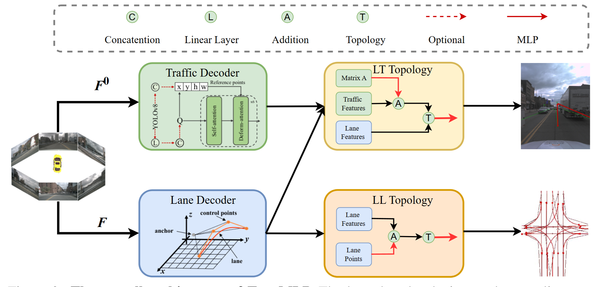
TopoMLP takes a set of multi-view images and produces four outputs at once — lane detection, traffic element detection, lane–lane topology, and lane–traffic topology. The flow is linear.
- Backbone & view transform — pass multi-view images through a backbone (ResNet-50 / Swin-B / VoVNet) to extract features.
- Lane Detector — a PETR-style 3D DETR decoder with position embedding extracts lane queries. Each lane query regresses the lane as Bézier control points.
- Traffic Element Detector — a Deformable-DETR decoder on the front-view features extracts traffic element queries.
- Topology Heads — feed the lane and traffic query features into two small MLP heads (one for lane–lane, one for lane–traffic) to predict relations.
The key point: the topology head consumes the detector’s query features as-is. There is no extra stage refining features for the relation, the way TopoNet does. The assumption — that pairing queries and pushing them through an MLP is enough once detection is good — is baked straight into the architecture.
① Lane Detector — representing a lane with Bézier control points
Regressing a lane directly as a sequence of points makes the output dimension grow with the number of points and destabilizes training. TopoMLP instead treats a lane as a Bézier curve. A curve is determined by a handful of control points, so the query only has to regress those. (This isn’t the first attempt at it, by the way. If you’re curious about a related paper, take a look at BeMapNet (CVPR 2023).)
📐 A quick aside — what is a Bézier curve?
A Bézier curve is a smooth parametric curve defined by a handful of control points. For a cubic Bézier, four control points $\mathbf{P}_0,\dots,\mathbf{P}_3$ are blended through the Bernstein polynomial basis to draw $\mathbf{B}(t)=\sum_{i=0}^{3}\binom{3}{i}(1-t)^{3-i}t^{i}\mathbf{P}_i,\; t\in[0,1]$. As $t$ flows from 0 to 1 the curve is traced out: it passes exactly through the start point ($\mathbf{P}_0$) and the end point ($\mathbf{P}_3$), but the interior control points only pull the curve toward themselves without ever being touched.
So how is this different from the usual approach? The most naive baseline is to directly regress an ordered list of $N$ points on the lane. But to represent a lane densely and smoothly you need a large $N$, which inflates the output dimension and makes optimization harder. Worse, there is no smoothness constraint between the points, so adjacent predicted points tend to jitter. A Bézier curve, by contrast, compresses the curve itself into just a few control points as its parameters.
That difference is exactly where the advantages come from. (1) It is compact — four control points fully determine the whole curve, so the output dim is small and fixed. (2) Smoothness comes for free — the curve is already analytically smooth, so there is no jitter. (3) It is resolution-independent — from the same control points you can later sample as many points as you like (e.g. 11). (4) It carries a strong shape prior that lanes are inherently smooth, which makes learning easier than fitting free points one by one. TopoMLP does exactly this: it predicts 4 control points (
num_reg_dim=12divided by $3$) and then expands them into 11 points via the Bernstein basis.
In code, the lane head regresses num_reg_dim values per lane, always a multiple of 3 (each control point is a 3D coordinate $(x, y, z)$). So the number of control points is num_reg_dim / 3.
# projects/topomlp/models/heads/lane_head.py
assert self.num_reg_dim % 3 == 0
self.num_control_points = int(self.num_reg_dim / 3)
By default num_reg_dim = 12, i.e. a lane is represented by 4 control points. When a lane later needs to be seen as “dense points” — for evaluation or topology — those 4 control points are expanded through the Bézier basis into 11 points.
# projects/topomlp/models/heads/topo_ll_head.py — control_points_to_lane_points()
from math import factorial   # imported at the top of the file

def comb(n, k):              # binomial nC k = n! / (k!(n-k)!), hand-rolled instead of math.comb
    return factorial(n) // (factorial(k) * factorial(n - k))

n_points = 11
n_control = lanes.shape[1]
A = np.zeros((n_points, n_control))
t = np.arange(n_points) / (n_points - 1)
for i in range(n_points):
    for j in range(n_control):
        A[i, j] = comb(n_control - 1, j) * np.power(1 - t[i], n_control - 1 - j) * np.power(t[i], j)
bezier_A = torch.tensor(A, dtype=torch.float32).to(lanes.device)
lanes = torch.einsum('ij,njk->nik', bezier_A, lanes)
Here comb is not a Python builtin but a binomial coefficient $\binom{n}{k}$ defined inside this function itself, and A is an $11 \times n_\text{control}$ Bernstein-basis matrix (the Bernstein basis is $b_{j,n}(t)=\binom{n}{j}(1-t)^{n-j}t^{j}$ — the weight each control point gets in the Bézier sum), and $t \in [0, 1]$ is split into 11 even steps to sample points on the curve. Control points are the compact representation used for learning and storage; the points are a derived representation recovered from them on demand.
The lane queries themselves are extracted PETR-style: a 3D position embedding is added to the multi-view features so each query is aware of its spatial location, then a DETR decoder refines the lane query set. The point is that they are position-aware — later, the topology head reuses that location information as a bonus.
② Traffic Element Detector
Traffic elements (lights, signs) are small 2D objects. So the traffic detector is just a standard 2D object detector — a Deformable-DETR decoder run on the front-view features, extracting 100 traffic queries. Nothing exotic; a well-proven choice.
The interesting part is the optional YOLOv8. Query-based detectors are weak on small objects and class imbalance, so the authors slot in proposals from an external YOLOv8 detector as anchor-box initialization to strengthen traffic detection. This is the very knob that tests the paper’s “detection sets the ceiling” claim — if you make the detector better, does topology follow?
The table answers it. On the same ResNet-50, turning YOLOv8 on (*) raises traffic detection $\text{DET}_t$, and that gain propagates straight into lane–traffic topology $\text{TOP}_{lt}$, lifting OLS too (paper Table 1).
| Method (R50) | $\text{DET}_t$ | $\text{TOP}_{lt}$ | OLS |
|---|---|---|---|
| TopoMLP | 50.0 | 22.8 | 38.2 |
TopoMLP* (+YOLOv8) |
53.3 | 30.1 | 41.2 |
A detection gain of $\text{DET}_t$ 50.0 → 53.3 pushes $\text{TOP}_{lt}$ from 22.8 → 30.1 (+7.3). The topology head is unchanged — only the detector got better, yet topology rose with it. That’s the cleanest one-line demonstration of the paper’s thesis. The same pattern holds on Swin-B ($\text{DET}_t$ 54.3 → 55.8, OLS 42.2 → 43.3).
③ Topology Head — two MLPs are all there is
Now the core. Once lane and traffic query features are ready, relations are predicted by two small MLP heads: TopoLLHead for lane–lane and TopoLTHead for lane–traffic. They are nearly identical, so we follow lane–lane.
The building block is a plain 3-layer MLP.
# projects/topomlp/models/heads/topo_ll_head.py
class MLP(nn.Module):
    def __init__(self, input_dim, hidden_dim, output_dim, num_layers):
        super().__init__()
        self.num_layers = num_layers
        h = [hidden_dim] * (num_layers - 1)
        self.layers = nn.ModuleList(nn.Linear(n, k) for n, k in zip([input_dim] + h, h + [output_dim]))

    def forward(self, x):
        for i, layer in enumerate(self.layers):
            x = F.relu(layer(x)) if i < self.num_layers - 1 else layer(x)
        return x
The head holds three of these — MLP_o1, MLP_o2 to embed each query (for lane–lane the two see the same lane queries, so they can be shared), and a classifier that turns a paired feature into a 0/1 relation.
# projects/topomlp/models/heads/topo_ll_head.py — __init__
self.MLP_o1 = MLP(in_channels_o1, in_channels_o1, 128, 3)
if shared_param:
    self.MLP_o2 = self.MLP_o1
else:
    self.MLP_o2 = MLP(in_channels_o2, in_channels_o2, 128, 3)
self.classifier = MLP(256, 256, 1, 3)
Follow the dimensions. MLP_o1 embeds a query feature to 128-d. For lane–lane, the two lane queries (start lane, end lane) are each embedded to 128-d, concatenated into a 256-d pair vector, and classifier collapses it to one logit. A sigmoid on that logit is the probability that the two lanes connect.
The forward shows exactly this.
# projects/topomlp/models/heads/topo_ll_head.py — forward()
o1_embeds = self.MLP_o1(o1_feat)
o2_embeds = self.MLP_o2(o2_feat)
if self.add_lane_pred:
    o1_embeds = o1_embeds + self.lane_mlp1(o1_pos)
    o2_embeds = o2_embeds + self.lane_mlp2(o2_pos)

num_query_o1 = o1_embeds.size(1)
num_query_o2 = o2_embeds.size(1)
o1_tensor = o1_embeds.unsqueeze(2).repeat(1, 1, num_query_o2, 1)
o2_tensor = o2_embeds.unsqueeze(1).repeat(1, num_query_o1, 1, 1)

relationship_tensor = torch.cat([o1_tensor, o2_tensor], dim=-1)
relationship_pred = self.classifier(relationship_tensor)
The crux is the four middle lines — pairwise broadcasting. Spread o1_embeds along one axis and o2_embeds along the other, concatenate, and you get a 256-d vector for every (lane $i$, lane $j$) pair at once. The output is therefore one logit per $N_{o1} \times N_{o2}$ pair — an adjacency matrix. No message passing, no iteration. Just one pass that forms every pair and runs it through an MLP.
The add_lane_pred branch is worth a look. When on, the query embedding gets the lane’s position (control points) added in through a separate MLP. For two lanes to connect, the endpoint of one must meet the start of the other in space — that geometric cue is injected straight into the feature. So TopoMLP’s reasoning isn’t only “feature similarity”; it is position-aware, looking at the geometry of the pair as well.
④ Loss — essentially identical to TopoNet
The relation loss is nothing new. Detection’s Hungarian matching picks out the queries that hit GT, GT adjacency is laid down as the label over pairs among them, and since connected pairs are a tiny fraction of this sparse graph, Focal Loss (gamma=2.0, alpha=0.25) tames the imbalance — mechanically the same as TopoNet’s Topology Loss. The full flow is already covered in the previous post’s Topology Loss, so we skip it.
Just one difference is worth noting. TopoNet applied the relation loss at every SGNN decoder layer, refining the relation layer by layer; TopoMLP has no graph and no iterative refinement, so the loss is applied once, on the final pair logits. The “simplicity” shows up even at the loss stage.
OpenLane-V2 Benchmark & Results
The benchmark and metric are the same as TopoNet’s — OpenLane-V2 and OLS (OpenLane-V2 Score). OLS aggregates four sub-metrics: lane detection $\text{DET}_l$, traffic element detection $\text{DET}_t$, lane–lane topology $\text{TOP}_{ll}$, and lane–traffic topology $\text{TOP}_{lt}$.
The square root on the topology terms is there because topology scores come out far lower than detection scores, so it balances the four metrics’ influence (the full definition is covered in the TopoNet post).
Here are the OpenLane-V2 subset-A numbers from paper Table 1.
| Method | Backbone | $\text{DET}_l$ | $\text{DET}_t$ | $\text{TOP}_{ll}$ | $\text{TOP}_{lt}$ | OLS |
|---|---|---|---|---|---|---|
| TopoNet | ResNet-50 | 28.5 | 48.1 | 4.1 | 20.8 | 35.6 |
| TopoMLP | ResNet-50 | 28.3 | 50.0 | 7.2 | 22.8 | 38.2 |
| TopoMLP* (+YOLOv8) | ResNet-50 | 28.8 | 53.3 | 7.8 | 30.1 | 41.2 |
| TopoMLP | Swin-B (48ep) | 32.5 | 53.5 | 11.9 | 29.4 | 43.7 |
At the same ResNet-50 and the same 24 epochs, TopoMLP beats TopoNet on OLS, 35.6 → 38.2. What’s worth noting is where the gap comes from.
- $\text{DET}_l$ is 28.5 vs 28.3 — essentially tied. Lane detection itself is comparable.
- But $\text{TOP}_{ll}$ jumps 4.1 → 7.2, nearly doubling. With no graph, just an MLP, lane–lane topology actually gets solved better.
Add YOLOv8 to strengthen traffic detection ($\text{DET}_t$ 50.0 → 53.3) and $\text{TOP}_{lt}$ leaps 22.8 → 30.1, pushing OLS to 41.2. This is the paper’s thesis showing up directly in the numbers: make the detector better and topology follows. Scale the backbone to Swin-B and train longer, and OLS reaches 43.7.
⚠️ Mind the metric version. OpenLane-V2’s TOP metric was redefined once (v1.0.0 → v2.x). The table above is all on the original (paper-era) metric; the latest numbers in the repo README — where the same model shows $\text{TOP}_{ll}$ in the 20s — are measured under a different metric version. Even for the same model, never compare numbers across metric versions. — but why was the version bumped at all? TopoMLP is part of that story.
Aside — a loophole in the TOP metric, and its fix
Separate from the “simple MLP” thesis, this is another contribution of TopoMLP. In §4.6 the authors point out that the original TOP metric itself has a loophole that lets you inflate the score for free.
First, how TOP is computed. For a lane (vertex) $v$, the predicted neighbor-edges are ranked by confidence (descending), and walking down the list you accumulate cumulative precision ($\text{precision}_i = \text{TP}_{\le i} / (\text{TP}_{\le i} + \text{FP}_{\le i})$). The score then averages the precision values at the positions where a TP lands. So the earlier a TP sits (fewer FPs ahead of it), the higher the score.
Here’s the hole. The detector doesn’t match every GT lane, and the metric defaults the edge confidence of unmatched instances to 1.0. So confidence-1.0 false positives sit at the very top of the ranking. Now — without touching the model — just binarize the predicted confidences around 0.5 ($> 0.5 \to 1.0$, $< 0.5 \to 0.0$): real TPs jump to 1.0 and rise to the same level as that unmatched-FP block instead of sitting below it. The TPs are no longer behind the FPs, cumulative precision rises, and TOP rises. No GT labels, no new predictive skill — pure metric gaming.
A small numeric example
Say vertex $v$ has 2 real GT neighbors ($\text{num\_gt}=2$). Four predicted edges survive the confidence $> 0.5$ filter:
| edge | raw conf | label | note |
|---|---|---|---|
| e1 | 1.0 | FP | unmatched instance — confidence defaulted to 1.0 |
| e2 | 1.0 | FP | unmatched instance — 〃 |
| e3 | 0.70 | TP | a genuine prediction (hits a real GT neighbor) |
| e4 | 0.60 | TP | 〃 |
Before — sorted by raw confidence (e1, e2, e3, e4):
| rank | edge | conf | label | TP | FP | precision |
|---|---|---|---|---|---|---|
| 1 | e1 | 1.00 | FP | 0 | 1 | 0 / 1 = 0.000 |
| 2 | e2 | 1.00 | FP | 0 | 2 | 0 / 2 = 0.000 |
| 3 | e3 | 0.70 | TP | 1 | 2 | 1 / 3 = 0.333 |
| 4 | e4 | 0.60 | TP | 2 | 2 | 2 / 4 = 0.500 |
My genuine edges e3·e4 (the correct answers) have lower confidence than the wrong e1·e2, so they sit behind them in the ranking. Their positions get low precision, and AP is low.
Now the trick — snap your predicted confidences around 0.5 ($> 0.5 \to 1.0$): e3, e4’s conf rises 0.70·0.60 → 1.00 and ties with e1, e2 (the predictions are unchanged — only the numbers move). Tie order is decided by the sort’s tie-break, so we look at both cases.
After (best case) — your TPs ahead of the tied FPs:
| rank | edge | conf | label | TP | FP | precision |
|---|---|---|---|---|---|---|
| 1 | e3 | 1.00 | TP | 1 | 0 | 1 / 1 = 1.000 |
| 2 | e4 | 1.00 | TP | 2 | 0 | 2 / 2 = 1.000 |
| 3 | e1 | 1.00 | FP | 2 | 1 | 2 / 3 = 0.667 |
| 4 | e2 | 1.00 | FP | 2 | 2 | 2 / 4 = 0.500 |
After (worst case) — tied FPs first (same order as Before):
$\text{AP}_\text{after}^\text{worst} = 5/12 \approx 0.417$ (unchanged from Before)
So $\text{AP}_\text{after} \in [0.417,\ 1.000]$ — with nothing newly predicted correctly, a single vertex gains up to +0.583 for free, and never loses in the worst case. The gain coming out as a range is the essence of the loophole: snapping lifts your TPs to the same level as the 1.0 unmatched-FP block so they no longer sit below it (the paper says “prior to some false positives”). Paper Table 4 shows the trick actually inflates $\text{TOP}_{ll}$ from 4.0 → 11.5 (+7.5) for TopoNet and 7.2 → 19.0 (+11.8) for TopoMLP.
How it was fixed — the actual code (v1.0.0 → v2.x)
The loophole lived in the official OpenLane-V2 devkit. In v1.0.0 (the version the paper used), the topology scorer’s caller only filters predicted edges by confidence $> 0.5$ and feeds the vertex indices straight in, so an unmatched detection’s (1.0) edge rides into the ranking.
# OpenLane-V2 v1.0.0 — openlanev2/evaluation/evaluate.py
THRESHOLD_RELATIONSHIP_CONFIDENCE = 0.5

def _AP_directerd(gts, preds):
    indices = np.arange(gts.shape[0])
    acc = []
    for gt, pred in zip(gts, preds):
        gt = indices[gt.astype(bool)]
        confidence = pred[pred > THRESHOLD_RELATIONSHIP_CONFIDENCE]
        pred = indices[pred > THRESHOLD_RELATIONSHIP_CONFIDENCE]   # scored as-is, no GT-match realignment
        acc.append(_average_precision_per_vertex(gt, pred, confidence))
    # ... same for the other (transpose) direction ...
    return acc
In v2.x the metric was revised. The scorer (_average_precision_per_vertex) is unchanged, but the stage above it, _mAP_topology_lclc, now — before scoring — realigns the predicted topology onto the lanes that detection matched to GT (idx_match_gt), and fills every unmatched slot with a guaranteed-wrong default (1 - gt) * (0.5 + eps).
# OpenLane-V2 v2.1.0 — openlanev2/centerline/evaluation/evaluate.py
def _mAP_topology_lclc(gts, preds, distance_thresholds):
    ...
    idx_match_gt = preds[token][f'lane_centerline_{distance_threshold}_idx_match_gt']
    gt_pred = {m: i for i, m in enumerate(idx_match_gt) if not np.isnan(m)}   # detection-matched lanes only

    gt_indices  = np.array(list(gt_pred.keys())).astype(int)
    pred_indices = np.array(list(gt_pred.values())).astype(int)
    preds_topology_lclc = np.ones_like(gts_topology_lclc) * np.nan
    xs = gt_indices[:, None].repeat(len(gt_indices), 1)
    ys = gt_indices[None, :].repeat(len(gt_indices), 0)
    preds_topology_lclc[xs, ys] = preds_topology_lclc_unmatched[pred_indices][:, pred_indices]
    # key: pin every unmatched slot to a guaranteed-wrong default
    preds_topology_lclc[np.isnan(preds_topology_lclc)] = (
        1 - gts_topology_lclc[np.isnan(preds_topology_lclc)]) * (0.5 + np.finfo(np.float32).eps)
    acc.append(_AP_directerd(gts=gts_topology_lclc, preds=preds_topology_lclc))
Why this kills the trick: the inflatable high-confidence edges of unmatched detections no longer enter the ranking at all. Only detection-matched lanes’ real edges are ranked at their true confidence; the rest are pinned to the default. Where GT = 0 that default is $0.5 + \text{eps}$ — barely over the threshold, a weak FP at the bottom of the ranking; where GT = 1 it is $0.0$ — below the threshold, so it’s dropped as a miss. Either way the default is wrong relative to GT, so there’s nothing left to game upward.
The paper’s own TOP† (Eq. 8)
If the v2.x code is OpenLane-V2’s official response, the paper proposed its own fix — a $\text{TOP}^\dagger$ with a correctness factor multiplied in.
$N_{TP}$, $N_{FP}$ are the counts of true / false positives. Because the factor depends on counts, not order, no amount of reranking changes it — snapping confidences to inflate the cumulative-precision term is capped by how many predictions are actually correct. (From the paper text alone it isn’t fully pinned whether $N_{TP}/N_{FP}$ are global or per-vertex counts; the reorder-invariance argument holds cleanly under the global reading.)
Table 4 is the evidence. Under the original metric the “enhance” trick lifts $\text{TOP}_{ll}$ by +7.5 to +11.8 for free; under $\text{TOP}^\dagger$ the same trick instead slightly drops the score (TopoNet $2.0 \to 1.0$, TopoMLP $4.5 \to 1.9$). The trick no longer working is exactly the proof the correctness factor closes the hole.
Note that the paper’s $\text{TOP}^\dagger$ (Eq. 8) and the devkit v2.x revision are two different fixes for the same loophole. $\text{TOP}^\dagger$ is a scalar correctness factor multiplied onto the score; the v2.x code realigns the candidate set to GT-matched lanes and overwrites the rest with a wrong default before scoring. The v2.x code does not implement Eq. 8 verbatim. And this is the root reason the same model gives different TOP numbers under v1.0.0 vs v2.1.0.
Conclusion — why simplicity wins
To sum up, TopoMLP’s contribution is this.
The ceiling on topology score is set by detection quality, not the reasoning module. So make the detector strong, solve relations with a simple position-aware MLP, and you still get SOTA.
Where TopoNet tries to solve relations with graph reasoning, TopoMLP answers “if detection is good in the first place, pairing queries and feeding them to an MLP is enough” — and that simple structure actually scores higher.
One caveat is worth stating, though. The way the paper argues “an MLP is enough” is less a clean one-to-one swap of GNN for MLP under identical conditions, and more an experiment showing how well topology is solved once detection is frozen to GT. So rather than the strong conclusion “reasoning isn’t needed,” the accurate reading is “in the current setting, the bottleneck is detection, not reasoning.” Also, in code, options like is_detach and add_lane_pred can differ between their defaults and the config values, so check the config directly when reproducing.
Even so, the message is clear and useful — if you want to raise topology, look at the detector before designing a fancier graph. If TopoNet defined the problem, TopoMLP re-pointed at what the real bottleneck in that problem is.
Thanks for reading. If I’ve misunderstood anything, please let me know :)
comments