TopoNet — Graph-based Topology Reasoning for Driving Scenes
Paper review · the first end-to-end framework and dataset that reason about how lanes connect — to each other, and to traffic elements.
각 figure의 출처는 하이퍼링크로 달아두었습니다 :)
+++ Lane Topology Reasoning 섹션의 첫 글이다. 이쪽 분야가 제대로 탐구되기 시작한 것이 CVPR 2023에서 열린 Autonomous Driving Challenge for Lane Topology 때부터인데, 해당 챌린지에서 나온 데이터셋이 OpenLane(현재 Lane Topology Reasoning 분야에서 계속 사용되고 있는 데이터셋), Baseline 모델이 TopoNet이다. TopoNet이 어떤 철학으로 모델을 설계했는지 주의깊게 관찰해보자! 🚀
TopoNet: Graph-based Topology Reasoning for Driving Scenes
Authors : Tianyu Li, Li Chen, Huijie Wang, Yang Li, Jiazhi Yang, Xiangwei Geng, Shengyin Jiang, Yuting Wang, Hang Xu, Chunjing Xu, Junchi Yan, Ping Luo, Hongyang Li (OpenDriveLab)
Venue : arXiv 2023
Paper Link : https://arxiv.org/abs/2304.05277
Code : https://github.com/OpenDriveLab/TopoNet
Introduction & Motivation
왜 Topology인가?
Online Mapping을 공부하다 보면, Lane Divider만 Detection하는 것에 의문이 생긴다. 자율주행의 최종 Downstream task인 Planning 관점에서 보면, 차량이 실제로 따라가야 하는 것은 divider가 아니라 그 사이의 space, 즉 Centerline이다. 게다가 직진만 할 게 아니라면, drivable한 Centerline들이 서로 어떻게 이어지는지 — 그 Topology를 이해하는 일이 무엇보다 중요해진다.
간단히 말해, “차선이 여기 있다”를 아는 것으로는 부족하다. 진짜로 필요한 건 “지금 이 lane에서 어디로 진입할 수 있는가”, 그리고 “저 신호등·표지판이 어느 lane을 통제하는가” 같은 Topology다.
기존의 Online HD Map Construction 계열(HDMapNet, MapTR, VectorMapNet 등)은 lane, lane divider, crosswalk 같은 map element를 detection하는 데 집중했다. 이렇게 detect된 element들 사이의 topology는 명시적으로 다루지 않거나, post-processing으로 heuristic하게 붙이는 경우가 많았다.
TopoNet은 detection에서 멈추지 않고, 다음 네 가지를 하나의 end-to-end framework에서 동시에 푼다.
- Lane Centerline Detection — lane의 centerline(directed)을 detect
- Traffic Element Detection — 신호등, 표지판 등 traffic element를 detect
- Lane-Lane Topology — lane과 lane이 어떻게 이어지는지 (진입/분기/합류)
- Lane-Traffic Topology — 어떤 traffic element가 어떤 lane을 통제하는지
저자들은 이를 두고 “abstracting traffic knowledge beyond conventional perception tasks” 라고 표현한다. 즉, perception을 넘어선 reasoning이 핵심이다.
왜 Centerline인가? (vs. Lane Divider)
앞서 설명한대로, 기존 mapping 논문들이 주로 다루던 것은 lane divider였다. 반면 topology를 다루려면 lane centerline이 더 적합하다.
이유는 간단하다. lane divider는 “space를 나누는 선”일 뿐, direction이나 connectivity를 직접 담지 못한다. 반면 centerline은 directed path로 볼 수 있어서, 한 centerline의 endpoint가 다른 centerline의 start point와 이어진다는 식으로 graph의 edge를 자연스럽게 정의할 수 있다.
즉, centerline을 node로 그 connection을 edge로 보면, drivable한 path 전체가 하나의 directed graph로 정리된다. topology reasoning은 여기서 시작한다.
Method
전체 파이프라인 개요
TopoNet의 큰 그림은 다음과 같다.
- Feature Extraction — Lane은 BEV space에서, traffic element는 PV space에서 detect하기 위해 BEV feature와 front-view PV feature를 따로 뽑는다.
- Query 기반 Detection — DETR-style로 lane query와 traffic query를 두고, 각각 centerline과 traffic element를 decode한다.
- Scene Graph Neural Network (SGNN) — detect된 query들을 node로 삼아, 그들 사이의 relation을 graph 위에서 message passing으로 update한다. 이 부분이 TopoNet의 핵심 contribution이다.
- Topology Head — update된 feature로부터 lane-lane, lane-traffic connection을 predict한다.
Scene Graph Neural Network (SGNN)
SGNN의 아이디어는 한 문장으로 요약된다. “각 lane의 feature를, 이어진 neighbor lane과 그 lane을 통제하는 traffic element의 정보로 enrich하자.”
기존 방식(STSU, TPLR)의 한계는, 각 element를 독립적으로 decode한 뒤 마지막에 relation만 따로 predict한다는 점이었다. 따라서 element feature 자체에는 “내가 누구와 이어져 있는가”라는 맥락이 들어있지 않다.
① Embedding — 2D와 3D를 같은 space로
본격적인 message passing에 앞서 짚을 문제가 하나 있다. TopoNet은 lane(LC)과 traffic element(TE)를 두 개의 parallel branch로 decode하는데, 둘의 feature space가 애초에 다르다. TE는 front-view image에서 나오는 2D query이고, LC는 BEV space의 3D(directed centerline) query다. coordinate frame도 dimension도 다른 둘을 같은 graph에 올려 “이 신호등이 이 lane을 통제한다”를 reasoning하려면, 먼저 공통 feature space로 align해야 한다.
그래서 각 decoder layer마다 TE query를 embedding network에 통과시켜 LC와 align되는 space로 변환한다 (Eq 1):
실제 구현은 projects/toponet/models/dense_heads/toponet_head.py의 te_embed_branch로, 2-layer MLP다:
# projects/toponet/models/dense_heads/toponet_head.py
# TE query를 LC와 같은 space로 보내는 embedding network
# (embed_dims=256 → 512 → 256)
te_embed_branch = nn.Sequential(
    nn.Linear(embed_dims, 2 * embed_dims),
    nn.ReLU(),
    nn.Dropout(0.1),
    nn.Linear(2 * embed_dims, embed_dims),
)
# 이 branch를 decoder layer 수만큼 복제해 layer별 독립 embedding을 만든다
self.te_embed_branches = _get_clones(te_embed_branch, num_decoder_layers)

# forward: layer(lid)마다 자기 전용 embedding으로 TE feature를 변환
te_feats = torch.stack([self.te_embed_branches[lid](te_feats[lid])
                        for lid in range(len(te_feats))])
한 가지 디테일 — 이렇게 변환된 $\tilde{Q}_t$는 SGNN 안에서 update하지 않고 그대로 둔다(intact). centerline으로부터 traffic element를 거꾸로 상상하는 것은 어렵고, TE feature를 너무 많이 건드리면 오히려 성능이 떨어진다는 것을 저자들이 실험적으로 확인했기 때문이다. 즉 정보는 TE → LC 방향으로 흐른다.
② Graph message passing — relation으로 feature 보강
이제 두 query가 같은 space에 놓였다. 앞서 말한 각 element를 독립적으로 decode하던 기존 방식과 달리, SGNN은 relation 정보를 feature를 만드는 과정 안으로 끌어들인다. 그런데 본격적으로 들어가기 전에, “graph”라는 말부터 정리하고 가자.
graph는 보통 $G = (V, E)$로 쓴다. $V$(vertices)는 node의 set, $E$(edges)는 edge의 set — 즉 “어떤 점들이 있고, 그 점들이 어떻게 연결되는가”다. TopoNet에서 node는 두 종류다.
- $V_l$ — lane(LC) node set. node 하나가 directed centerline 하나다.
- $V_t$ — traffic element(TE) node set. node 하나가 신호등·표지판 하나(2D box)다.
가장 단순하게는 모든 node를 한 graph에 넣고 다 이어버릴 수 있다 — $V = V_l \cup V_t$에 edge를 $E \subseteq V \times V$로 두는 fully-connected graph다. ($V \times V$는 가능한 모든 node 쌍을 뜻하는 Cartesian product다.) 하지만 이러면 연산량이 커질 뿐 아니라, 사람이 임의로 세워둔 신호등 두 개 사이처럼 의미 없는 message까지 흐른다. 그래서 TopoNet은 의미 있는 relation만 남긴 두 개의 directed graph로 쪼갠다.
- $G_{ll}$ — lane–lane graph. node는 lane뿐, edge candidate는 모든 (lane, lane) 쌍($V_l \times V_l$)이다. “어느 lane이 어느 lane으로 이어지나”.
- $G_{lt}$ — lane–traffic graph. node는 lane과 traffic element, edge candidate는 (lane, traffic element) 쌍($V_l \times V_t$)뿐이다 — traffic element끼리는 잇지 않는다. “어느 신호·표지가 어느 lane을 통제하나”.
SGNN은 이 두 graph 위에서 각각 message를 propagate한 뒤, 두 결과를 합쳐 lane feature를 update한다. 이제 각 graph를 — 수식과 그에 대응하는 실제 코드를 나란히 두고 — 차례로 보자.
(a) lane–lane
각 layer는 이전 layer가 predict한 adjacency matrix $A_{ll}^{i-1}$로부터, message propagation을 제어하는 weight matrix $T_{ll}^{i}$를 만든다 (Eq 3):
여기서 $I$는 self-loop(자기 자신의 feature를 보존하는 identity matrix)이고, $A_{ll}^{i-1\top}$는 $A_{ll}^{i-1}$의 transpose(backward direction)다. centerline은 directed path라 message가 한 방향(lane → 후행 lane)으로만 흐르는데, lane의 위치는 neighbor의 위치를 알려주는 단서이므로 transpose를 더해 bidirectional 교류를 허용한다. $\beta_{ll}$은 propagation 비율을 조절하는 hyperparameter다.
$A_{ll}^{\top}$가 방향만 뒤집은 adjacency matrix임을 작은 예로 보자. lane 5개가 1→2→3, 4→5로 이어지고, convention은 $A[i][j]=1$이면 “$i$에서 $j$로 갈 수 있다”:
lane 2를 보면 — $A$의 2행 [0 0 1 0 0]은 다음 lane 3(successor), $A^{\top}$의 2행 [1 0 0 0 0]은 이전 lane 1(predecessor)을 가리킨다. forward($A$)만 쓰면 자기 successor만 보이므로, transpose를 더해 predecessor까지 bidirectional로 모은다.
코드로 보면 식 (3)이 거의 그대로 옮겨진다:
# sgnn_decoder.py · class LclcSkgGCNLayer
# input: lane feature [B,N,C],  adj: 이전 layer가 예측한 adjacency matrix A_ll [B,N,N]
def forward(self, input, adj):
    support_loop = torch.matmul(input, self.weight)          # self-loop → Eq 3의 I
    output = support_loop
    if self.edge_weight != 0:                                # edge_weight = β_ll
        support_forward = torch.matmul(input, self.weight_forward)
        output_forward = torch.matmul(adj, support_forward)              # A · X·W_f  (forward)
        output += self.edge_weight * output_forward

        support_backward = torch.matmul(input, self.weight_backward)
        output_backward = torch.matmul(adj.permute(0, 2, 1), support_backward)  # Aᵀ · X·W_b  (backward)
        output += self.edge_weight * output_backward
    return output
self.weight(self-loop)가 $I$ 항, adj/adj.permute가 $A_{ll}$과 $A_{ll}^{\top}$, edge_weight가 $\beta_{ll}$이다. forward와 backward를 각각 다른 weight($W_f, W_b$)로 처리하는 것이 Eq 3에서 두 항을 더하는 것과 대응한다.
(b) lane–traffic — transpose가 없는 이유
lane–traffic도 같은 방식이지만 한 군데가 다르다 (Eq 4):
$O$는 원소가 모두 0인 zero matrix(첫 layer는 relation을 모름)이고, $A_{lt}^{i-1}$는 (lane, traffic element) adjacency matrix다. lane–lane과 비교하면 transpose 항도 self-loop도 없다. $G_{lt}$가 bipartite graph이기 때문이다 — 한쪽엔 lane, 다른 쪽엔 traffic element만 있고, relation은 “traffic element → lane”이라는 한 방향뿐이다(lane이 신호등을 통제하지는 않으니까). 그래서 backward(transpose)도, 같은 종류끼리의 self-loop도 의미가 없다. 이 GCN의 실제 코드는 아래 ③에서 함께 본다 — vanilla(Eq 4)와 class별 버전(Eq 6)이 같은 함수에 들어 있기 때문이다.
③ Scene Knowledge Graph — traffic element를 class별로
여기까지가 논문이 Vanilla Scene Graph라 부르는 단계다. 그런데 한계가 하나 있다 — vanilla GCN은 connectivity만 보고 node의 종류(semantic)는 무시한다. “직진 표지판”과 “빨간 신호등”이 한 lane에 주는 의미는 전혀 다른데, 같은 weight로 섞으면 이 차이가 사라진다. 그래서 lane–traffic graph에는 traffic element를 class별로 다른 weight로 처리하는 Scene Knowledge Graph를 둔다 (Eq 6):
Eq 4와 비교하면 차이는 안쪽 합 $\sum_{c_t \in C_t}$ 하나다. $C_t$는 traffic element의 class set(신호등·표지판 등), $N(x)$는 lane $x$에 연결된 traffic element들, $S_t(c_t, y)$는 traffic element $y$가 class $c_t$일 classification score, $W_{lt}(c_t)$는 class $c_t$ 전용 weight다. 즉 vanilla의 single weight 자리에, class별 weight를 classification score로 가중해 더한 것이 들어간다.
이 class별 처리는 코드에서 바로 드러난다:
# sgnn_decoder.py · class LcteSkgGCNLayer
# self.weight: [num_te_classes, C, C]  ← class마다 별도 weight (Eq 6의 W_lt(c_t))
def forward(self, te_query, lcte_adj, te_cls_scores):
    cls_scores = te_cls_scores.detach().sigmoid().unsqueeze(3)   # S_t : per-class classification score
    te_feats = te_query.unsqueeze(2) * cls_scores                # TE feature를 class score로 가중
    te_feats = te_feats.permute(0, 2, 1, 3)                      # [B, num_class, num_te, C]

    support = torch.matmul(te_feats, self.weight).sum(1)         # per-class weight 적용 후 Σ_c_t (Eq 6 안쪽 합)
    adj = lcte_adj * self.edge_weight                            # β_lt · A_lt  (Eq 4, no transpose)
    output = torch.matmul(adj, support)                         # A_lt · (...)
    return output
self.weight가 class 축을 가진 [num_te_classes, C, C]이고, .sum(1)이 Eq 6의 안쪽 합 $\sum_{c_t}$다. cls_scores가 $S_t$, adj = lcte_adj * edge_weight가 Eq 4의 $\beta_{lt} A_{lt}$ — transpose가 없는 것까지 그대로 보인다. 즉 vanilla(Eq 4)와 knowledge graph(Eq 6)가 한 함수에 함께 구현돼 있다.
두 그래프를 합치기 (Eq 2)
두 GCN의 결과 $Q'_l$(lane–lane)과 $Q''_l$(lane–traffic)은 합쳐져 최종 lane feature가 된다 (Eq 2):
둘을 concat하고 ReLU·downsample로 한 dimension($R^i$, information gain)으로 줄인 뒤, 원래 query에 residual로 더한다. 코드에서도 같다:
# sgnn_decoder.py · class FFN_SGNN.forward  (한 SGNN layer의 합치기)
lclc_features = self.lclc_gnn_layer(out, lclc_adj)                      # Q'_l  (lane–lane GCN)
lcte_features = self.lcte_gnn_layer(te_query, lcte_adj, te_cls_scores)  # Q''_l (lane–traffic GCN)
out = torch.cat([lclc_features, lcte_features], dim=-1)                 # concat
out = self.downsample(self.activate(out))                              # ReLU → downsample = R^i
return identity + self.dropout_layer(out)                              # residual: Q_l + R^i
이 concat → downsample → residual이 Eq 2 그대로이고, 이것이 한 SGNN layer의 한 바퀴다.
Input과 Iterative Refinement
마지막으로 두 가지. Input — SGNN의 lane query는 DETR식 learnable query embedding으로, decoder에서 BEV feature와 cross-attention하며 lane 정보를 흡수한다. adjacency matrix는 input이 아니라 layer가 돌며 만들어지는 intermediate output이다.
Iteration — 그래서 첫 layer의 adjacency matrix는 0(relation 모름)으로 initialize되고, 이후 매 layer가 (relation으로 feature 보강) → (보강된 feature로 relation 재predict)을 한 번씩 수행해 다음 layer에 넘긴다. 이때 relation 재predict은 GCN이 아니라 별도의 pairwise MLP head(relationship_head.py)가 맡는다 — GCN이 relation을 소비해 feature를 만들고, head가 feature로 relation을 생산한다. 이 두 단계가 layer마다 반복되면서 detection과 relation이 같이 좋아진다. 이게 SGNN이 노린 구조다.
Topology Loss — sparse한 relation을 학습시키기
training loss는 detection(DET)과 topology(TOP)로 나뉜다. DET는 DETR 계열의 일반적인 classification+regression loss라 넘어가고, TOP loss만 짚자.
topology head는 두 instance feature를 받아 연결 여부(connected?)를 predict하는 binary classifier다. label은 perception head의 matching 결과를 기준으로 각 pair에 부여된다. 문제는 graph가 매우 sparse하다는 점이다 — $N$개 lane이면 가능한 pair는 $N^2$인데 실제 연결된 pair는 극소수라, positive(연결)/negative(비연결) sample이 극심하게 imbalance하다. 그래서 단순 BCE 대신 Focal Loss를 쓴다 — 수가 압도적인 easy negative의 비중을 낮추는 것이다. 이 loss는 매 decoder layer에 걸리므로, 앞서 본 iterative refinement와 함께 relation 예측이 layer마다 조금씩 나아진다.
OpenLane-V2 Benchmark & OLS Metric
TopoNet은 단순히 모델만 내놓은 게 아니라, 이 task를 평가하기 위한 benchmark OpenLane-V2와 함께 등장했다 (benchmark는 NeurIPS 2023 Datasets & Benchmarks 트랙에 별도로 발표됨).
evaluation metric OLS(OpenLane-V2 Score)는 네 가지 sub-metric의 종합이다.
- DET$_l$ — lane centerline detection accuracy
- DET$_t$ — traffic element detection accuracy
- $\text{TOP}_{ll}$ — lane-lane topology accuracy
- $\text{TOP}_{lt}$ — lane-traffic topology accuracy
topology 항에 square root가 붙는 이유는, topology score가 detection score보다 일반적으로 훨씬 낮게 나오기 때문이다(relation reasoning이 detection보다 어렵다). square root로 scale을 끌어올려 네 metric이 비슷한 영향력을 갖도록 balance를 맞춘 것이다.
결과
OpenLane-V2 subset-A 기준, TopoNet의 수치는 다음과 같다 (paper Table 1).
| Metric | Value |
|---|---|
| OLS | 35.6 |
| DET$_l$ (centerline) | 28.5 |
| DET$_t$ (traffic element) | 48.1 |
| $\text{TOP}_{ll}$ (lane-lane) | 4.1 |
| $\text{TOP}_{lt}$ (lane-traffic) | 20.8 |
핵심은 절대 수치 자체보다, topology metric($\text{TOP}_{ll}$, $\text{TOP}_{lt}$)에서 기존 mapping 계열(MapTR, VectorMapNet 등)을 큰 폭으로 앞섰다는 점이다. detection만 잘하던 기존 model들과 달리, relation reasoning을 설계에 직접 넣은 것이 이 격차로 이어졌다.
다만 $\text{TOP}_{ll}$이 4.1에 불과하다는 점은, lane-lane topology가 여전히 매우 어려운 open problem이라는 것도 동시에 보여준다. 이 지점이 이후 후속 연구들이 파고드는 틈이 된다.
Conclusion — 그리고 왜 이 글이 먼저인가
정리하면, TopoNet의 기여는 이렇다.
lane·traffic element detection과 그들 사이의 relation reasoning을, 별개의 단계가 아니라 하나의 graph 위에서 end-to-end로 묶은 첫 framework.
기존 Online Mapping이 “무엇이 어디 있는가”까지 풀었다면, TopoNet은 “그것들이 어떻게 이어지는가”를 더한 셈이다. detect한 map을 실제 주행에 쓰려면 이 relation이 결국 필요하다.
이 글을 Lane Topology Reasoning 섹션의 첫 글로 둔 이유가 여기에 있다. 이후에 다룰 TopoMLP(graph 대신 강한 detection + 단순한 MLP topology head로 더 좋은 성능을 낸다는 반박)도 TopoNet이 정의한 문제 설정 위에서 출발한다.
다음 글에서는 그중 TopoMLP를 다뤄보려 한다.
읽어주셔서 감사합니다. 혹시 제가 잘못 이해한 부분이 있다면 언제든 알려주세요 :)
Sources for each figure are linked inline :)
Once you spend enough time studying Online Mapping, a question creeps in: is it really enough to only detect centerlines? From a planning standpoint —
+++ This is the first post in the Lane Topology Reasoning section. After reading through a stack of Online HD Map Construction papers, I came to feel that good perception alone isn’t enough — you have to solve the *relationships (topology), like “can I actually go from this lane to that one,” before a map becomes something you can really drive on. TopoNet felt like the natural starting point for that, so I picked it as the first post 🚀*
TopoNet: Graph-based Topology Reasoning for Driving Scenes
Authors : Tianyu Li, Li Chen, Huijie Wang, Yang Li, Jiazhi Yang, Xiangwei Geng, Shengyin Jiang, Yuting Wang, Hang Xu, Chunjing Xu, Junchi Yan, Ping Luo, Hongyang Li (OpenDriveLab)
Venue : arXiv 2023
Paper Link : https://arxiv.org/abs/2304.05277
Code : https://github.com/OpenDriveLab/TopoNet
Introduction & Motivation
Why topology?
In an autonomous-driving stack, a map’s job doesn’t end at knowing “a lane is here.” What you actually need are the relationships: “from this lane, where can I go next?” and “which lane does that traffic light / sign govern?”
Prior Online HD Map Construction methods (HDMapNet, MapTR, VectorMapNet, etc.) focused on detecting map elements — lanes, dividers, crosswalks. But the connectivity (topology) between those detected elements was either left implicit or stitched on afterwards with hand-crafted post-processing heuristics.
TopoNet doesn’t stop at detection — it solves the following four jointly, in a single end-to-end framework:
- Lane Centerline Detection — detect directed lane centerlines
- Traffic Element Detection — detect traffic lights, signs, and other elements
- Lane-Lane Topology — how lanes connect to each other (merge / split / continue)
- Lane-Traffic Topology — which traffic element governs which lane
The authors describe this as “abstracting traffic knowledge beyond conventional perception tasks.” In other words, the key is reasoning that goes beyond perception.
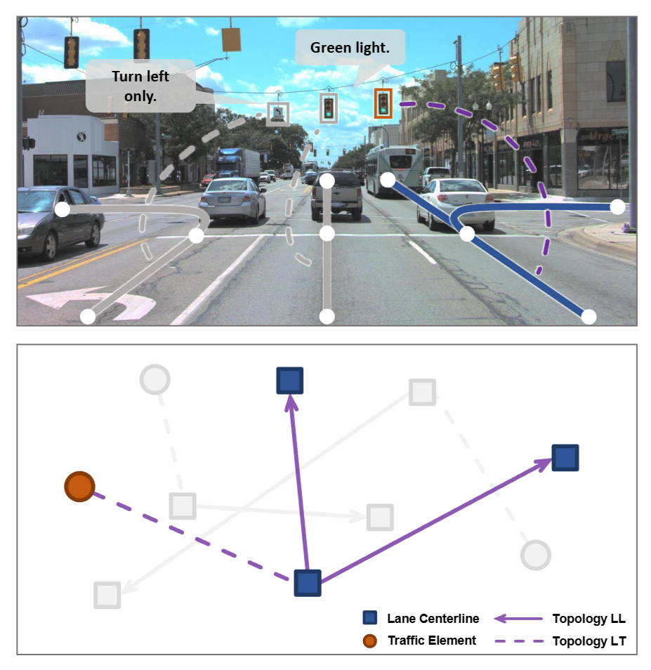
Fig 1. TopoNet reasons about lane–lane / lane–traffic relations as a graph (see Fig. 1 of the paper)
Why centerlines? (vs. lane dividers)
One point worth pausing on: earlier mapping papers mostly dealt with lane dividers (the boundary lines). For topology, however, lane centerlines are the better primitive.
The reason is simple. A divider is just “a line that splits space” — it doesn’t directly carry direction or connectivity. A centerline, on the other hand, can be seen as a directed path, so you can naturally define a graph edge by saying “the endpoint of one centerline connects to the start of another.”
Treat centerlines as nodes and their connections as edges, and the drivable routes form a single directed graph. Topology reasoning starts here.
Method
Pipeline overview
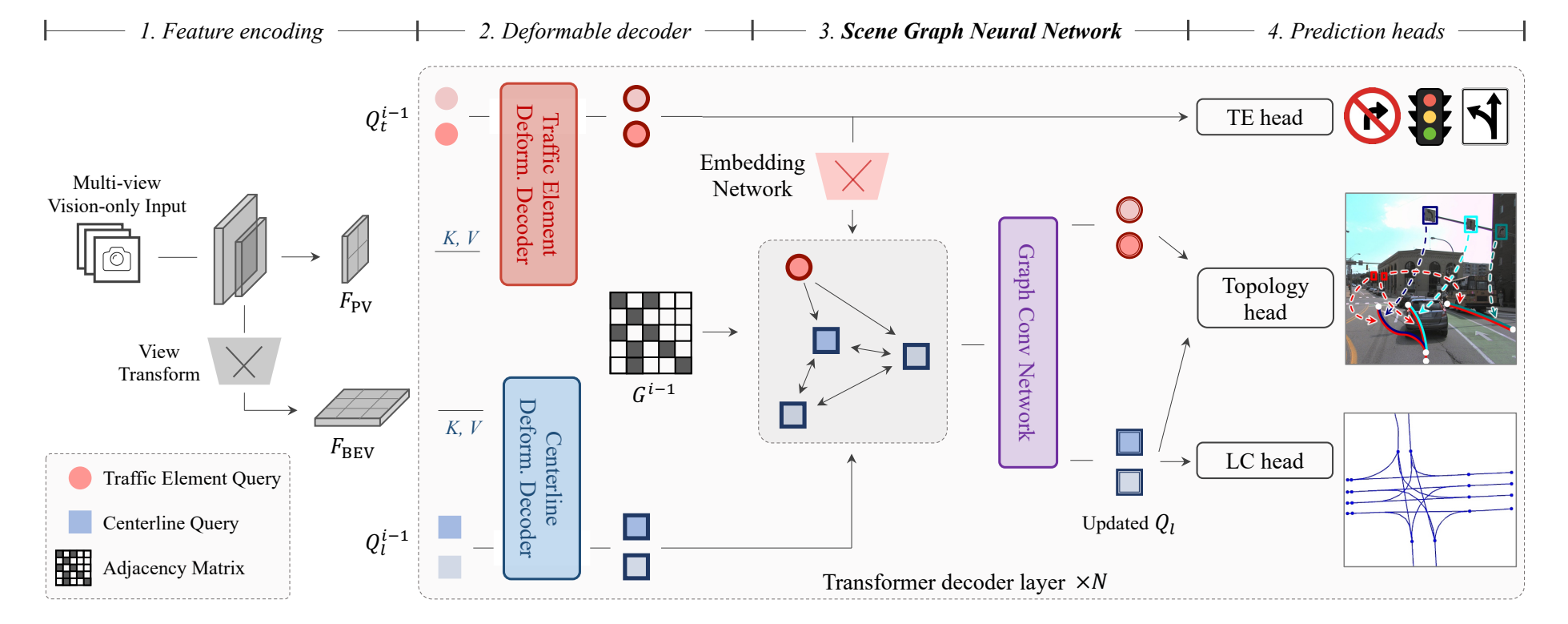
The big picture of TopoNet looks like this:
- Feature Extraction — from multi-view camera images, extract both BEV (Bird’s-Eye-View) and PV (Perspective-View) features. Lanes are naturally detected in BEV space, traffic elements in the perspective (PV) image.
- Query-based Detection — following the DETR family, use lane queries and traffic queries to decode centerlines and traffic elements respectively.
- Scene Graph Neural Network (SGNN) — treat the detected queries as nodes and update their features through message passing over a graph. This is TopoNet’s core contribution.
- Topology Head — from the updated features, predict lane-lane and lane-traffic connectivity.
Scene Graph Neural Network (SGNN)
The idea behind SGNN fits in one sentence: “enrich each lane’s feature with information from its connected neighbor lanes and from the traffic elements that govern it.”
The limitation of prior approaches was that each element was decoded independently, with the relationships predicted only at the very end. That leaves the element features themselves without any context about “who am I connected to.”
① Embedding — putting 2D and 3D in one space
Before any message passing, there’s a problem to settle. TopoNet decodes lanes (LC) and traffic elements (TE) as two parallel branches, but their feature spaces differ to begin with. TE is a 2D query detected in the front-view image; LC is a 3D query (directed centerline) in BEV space. To put two things of different coordinate frames and dimensions on one graph and reason “this light governs this lane,” they must first be aligned into a common feature space.
So at each decoder layer, the TE query is passed through an embedding network that maps it into a space matched to LC Eq 1:
The implementation is te_embed_branch in projects/toponet/models/dense_heads/toponet_head.py — a 2-layer MLP:
# projects/toponet/models/dense_heads/toponet_head.py
# embedding network that sends TE queries into LC's space
# (embed_dims=256 -> 512 -> 256)
te_embed_branch = nn.Sequential(
    nn.Linear(embed_dims, 2 * embed_dims), nn.ReLU(), nn.Dropout(0.1),
    nn.Linear(2 * embed_dims, embed_dims),
)
# clone it per decoder layer so each layer gets its own embedding
self.te_embed_branches = _get_clones(te_embed_branch, num_decoder_layers)

# forward: embed each decoder layer's TE features with that layer's own branch
te_feats = torch.stack([self.te_embed_branches[lid](te_feats[lid])
                        for lid in range(len(te_feats))])
One detail — the embedded $\tilde{Q}_t$ is then kept intact inside the SGNN. Imagining traffic elements back from centerlines is hard, and the authors empirically found that touching TE features too much actually hurts. Information flows from TE to LC.
② Graph message passing — refining features with relations
Now that both queries live in the same space, here’s the main part. Unlike the earlier approaches that decode each element independently, SGNN pulls relational information into the feature-building process itself. But before diving in, let’s pin down the word “graph.”
A graph is written $G = (V, E)$, where $V$ (vertices) is the set of nodes and $E$ (edges) the set of connections — “what points exist, and how are they linked.” In TopoNet the nodes come in two kinds.
- $V_l$ — the lane (LC) nodes. One node = one directed centerline.
- $V_t$ — the traffic-element (TE) nodes. One node = one light/sign (a 2D box).
The naive option is to drop every node into one graph and connect them all — a fully-connected graph with $V = V_l \cup V_t$ and edges $E \subseteq V \times V$. ($V \times V$ is the Cartesian product: every possible pair of nodes.) But that’s expensive and lets meaningless messages flow — e.g. between two traffic lights placed arbitrarily by humans. So TopoNet splits it into two directed graphs that keep only the meaningful relations:
- $G_{ll}$ — the lane–lane graph. Nodes are lanes only; candidate edges are all (lane, lane) pairs ($V_l \times V_l$). “Which lane leads to which.”
- $G_{lt}$ — the lane–traffic graph. Nodes are lanes and traffic elements; candidate edges are only (lane, traffic-element) pairs ($V_l \times V_t$) — never element-to-element. “Which light/sign governs which lane.”
SGNN propagates messages over both graphs, then merges the two results to update the lane features. Let’s take each graph in turn, putting the equation and its actual code side by side.
(a) lane–lane
Each layer turns the adjacency $A_{ll}^{i-1}$ predicted by the previous layer into a weight matrix $T_{ll}^{i}$ that controls message flow (Eq 3):
Here $I$ is the self-loop (the identity matrix, preserving a node’s own feature), and $A_{ll}^{i-1\top}$ is the transpose (backward direction) of $A_{ll}^{i-1}$. Because a centerline is a directed path, messages flow one way (lane → successor); but a lane’s position cues its neighbors’, so the transpose is added for two-way exchange. $\beta_{ll}$ controls how much is propagated.
A small example shows $A_{ll}^{\top}$ is just the adjacency with its direction flipped. Say five lanes connect as 1→2→3 and 4→5, with the convention $A[i][j]=1$ meaning “you can go from $i$ to $j$“:
Take lane 2 — row 2 of $A$, [0 0 1 0 0], points to its successor 3; row 2 of $A^{\top}$, [1 0 0 0 0], points to its predecessor 1. Forward ($A$) alone only sees successors, so the transpose is added to gather predecessors too.
In code, Eq 3 carries over almost verbatim:
# sgnn_decoder.py · class LclcSkgGCNLayer
# input: lane feature [B,N,C],  adj: prev layer's adjacency A_ll [B,N,N]
def forward(self, input, adj):
    support_loop = torch.matmul(input, self.weight)          # self-loop → the I in Eq 3
    output = support_loop
    if self.edge_weight != 0:                                # edge_weight = β_ll
        support_forward = torch.matmul(input, self.weight_forward)
        output_forward = torch.matmul(adj, support_forward)              # A · X·W_f  (forward)
        output += self.edge_weight * output_forward

        support_backward = torch.matmul(input, self.weight_backward)
        output_backward = torch.matmul(adj.permute(0, 2, 1), support_backward)  # Aᵀ · X·W_b  (backward)
        output += self.edge_weight * output_backward
    return output
self.weight (self-loop) is the $I$ term, adj / adj.permute are $A_{ll}$ and $A_{ll}^{\top}$, and edge_weight is $\beta_{ll}$. Handling forward and backward with separate weights ($W_f, W_b$) mirrors summing the two terms in Eq 3.
(b) lane–traffic — why there’s no transpose
lane–traffic works the same way, with one difference (Eq 4):
$O$ is the all-zeros matrix (the first layer knows no relations), and $A_{lt}^{i-1}$ is the (lane, traffic-element) adjacency. Compared to lane–lane, there’s no transpose and no self-loop. The reason is that $G_{lt}$ is bipartite — one side is lanes, the other traffic elements, and the relation is one-directional, “traffic element → lane” (a lane doesn’t govern a light). So a reverse direction and a same-type self-loop are both meaningless. We’ll see this GCN’s code in ③ below — vanilla (Eq 4) and the per-class version (Eq 6) live in the same function.
③ Scene Knowledge Graph — traffic elements, per class
Everything so far is what the paper calls the Vanilla Scene Graph. But it has a gap: vanilla GCN looks only at connectivity and ignores a node’s type (semantics). A “go-straight sign” and a “red light” mean very different things to a lane, yet mixing them with the same weight erases that difference. So the lane–traffic graph uses a Scene Knowledge Graph that weights traffic elements per class (Eq 6):
Compared to Eq 4, the one difference is the inner sum $\sum_{c_t \in C_t}$. $C_t$ is the set of traffic-element classes (lights, signs, …), $N(x)$ the traffic elements connected to lane $x$, $S_t(c_t, y)$ the score that element $y$ is class $c_t$, and $W_{lt}(c_t)$ a per-class weight. So in place of vanilla’s single weight, the per-class weights summed and scored by classification go in.
The code makes this per-class handling explicit:
# sgnn_decoder.py · class LcteSkgGCNLayer
# self.weight: [num_te_classes, C, C]  ← one weight per class (W_lt(c_t) in Eq 6)
def forward(self, te_query, lcte_adj, te_cls_scores):
    cls_scores = te_cls_scores.detach().sigmoid().unsqueeze(3)   # S_t : per-class scores
    te_feats = te_query.unsqueeze(2) * cls_scores                # scale TE features by class score
    te_feats = te_feats.permute(0, 2, 1, 3)                      # [B, num_class, num_te, C]

    support = torch.matmul(te_feats, self.weight).sum(1)         # per-class weight, then Σ_c_t (Eq 6 inner sum)
    adj = lcte_adj * self.edge_weight                            # β_lt · A_lt  (Eq 4, no transpose)
    output = torch.matmul(adj, support)                         # A_lt · (...)
    return output
self.weight carries a class axis [num_te_classes, C, C], and .sum(1) is the inner sum $\sum_{c_t}$ of Eq 6. cls_scores is $S_t$, and adj = lcte_adj * edge_weight is the $\beta_{lt} A_{lt}$ of Eq 4 — with no transpose, just as stated. So vanilla (Eq 4) and the knowledge graph (Eq 6) live in one function.
Merging the two graphs (Eq 2)
The two GCN outputs $Q'_l$ (lane–lane) and $Q''_l$ (lane–traffic) are merged into the final lane feature (Eq 2):
Concatenate the two, reduce to one dimension ($R^i$, the information gain) via ReLU + downsample, and add back to the original query as a residual. The code matches:
# sgnn_decoder.py · class FFN_SGNN.forward  (merging within one SGNN layer)
lclc_features = self.lclc_gnn_layer(out, lclc_adj)                      # Q'_l  (lane–lane GCN)
lcte_features = self.lcte_gnn_layer(te_query, lcte_adj, te_cls_scores)  # Q''_l (lane–traffic GCN)
out = torch.cat([lclc_features, lcte_features], dim=-1)                 # concat
out = self.downsample(self.activate(out))                              # ReLU → downsample = R^i
return identity + self.dropout_layer(out)                              # residual: Q_l + R^i
This concat → downsample → residual is exactly Eq 2, and that is one turn of a single SGNN layer.
Input and iterative refinement
Two last points. Input — SGNN’s lane queries are DETR-style learned query embeddings that cross-attend to BEV features in the decoder to soak up lane information; the adjacency is not an input but an intermediate product built up across layers.
Refinement — so the first layer’s adjacency is initialized to 0 (relations unknown), and each subsequent layer does one round of (refine features with relations) → (re-predict relations) before handing off. The re-prediction isn’t the GCN but a separate pairwise MLP head (relationship_head.py) — the GCN consumes relations to build features, the head turns features into relations. These two steps repeat at every layer, and detection and relations improve together — which is the structure SGNN was built around.
Topology loss — learning a sparse relation
The training loss splits into detection (DET) and topology (TOP). DET is the usual DETR-style classification + regression loss, so we skip it and focus on the TOP loss.
The topology head is a binary classifier that takes two instance features and predicts whether they’re connected; ground truth is assigned per pair from the perception heads’ matching results. The catch is that the graph is very sparse — with $N$ lanes there are $N^2$ possible pairs but only a handful are actually connected, so positive/negative samples are wildly imbalanced. Hence Focal loss instead of plain BCE, to down-weight the overwhelming easy negatives. This supervision is applied at every decoder layer, dovetailing with the iterative refinement to sharpen relations layer by layer.
OpenLane-V2 Benchmark & OLS Metric
TopoNet didn’t just ship a model — it arrived together with OpenLane-V2, a benchmark for evaluating this task (the benchmark itself was published separately in the NeurIPS 2023 Datasets & Benchmarks track).
The evaluation metric, OLS (OpenLane-V2 Score), is a composite of four sub-metrics:
- DET$_l$ — lane centerline detection accuracy
- DET$_t$ — traffic element detection accuracy
- $\text{TOP}_{ll}$ — lane-lane topology accuracy
- $\text{TOP}_{lt}$ — lane-traffic topology accuracy
The square root on the topology terms is there because topology scores tend to come out much lower than detection scores (relational reasoning is harder than detection). Taking the square root lifts their scale so that all four sub-metrics carry comparable weight.
Results
On OpenLane-V2 subset-A, TopoNet’s numbers are (paper Table 1):
| Metric | Value |
|---|---|
| OLS | 35.6 |
| DET$_l$ (centerline) | 28.5 |
| DET$_t$ (traffic element) | 48.1 |
| $\text{TOP}_{ll}$ (lane-lane) | 4.1 |
| $\text{TOP}_{lt}$ (lane-traffic) | 20.8 |
What matters is not the absolute numbers but the fact that on the topology metrics ($\text{TOP}_{ll}$, $\text{TOP}_{lt}$) it beats the prior mapping line (MapTR, VectorMapNet, etc.) by a wide margin. Unlike prior models that were only good at detection, putting relational reasoning directly into the design is what produced this gap.
That said, a $\text{TOP}_{ll}$ of just 4.1 also shows that lane-lane topology remains a very hard open problem. That gap is exactly the opening that later work digs into.
Conclusion — and why this post comes first
To sum up, TopoNet’s contribution is this.
The first framework to bind lane/traffic-element detection and the reasoning about their relationships into a single graph, end-to-end, rather than as separate stages.
Earlier Online Mapping solved “what is where”; TopoNet adds “how those things connect.” To actually drive on a detected map, you end up needing that connectivity.
That is why this post opens the Lane Topology Reasoning section. TopoMLP — which I’ll cover next, a rebuttal arguing that strong detection plus a simple MLP topology head does even better than elaborate graph reasoning — also sets out from the problem formulation TopoNet defined.
In the next post, I’ll dig into TopoMLP.
Thanks for reading. If I’ve misunderstood anything, please don’t hesitate to let me know :)
comments